A Classification Analysis on Breast Cancer

September 27, 2023

It's nearly breast cancer awareness month. According to the World Health Organization (WHO), breast cancer is the "world's most prevalent cancer," affecting a cumulative 7.8 million people worldwide as of 2020. As you'll see in today's analysis, we are able to detect the malignancy of breast cancer tumors with a high degree of accuracy. Early detection is one of the best ways to increase survival rate, so don't wait and go see a doctor for a breast cancer screening test!

Okay so we're back in action, this time with a classification project. My innagural project was a regression analysis on Ethereum, during which I compared many different models and used a validation-set approach to identify the best performing model. Today's project will be very similar in that I will be fitting many different classification models to the training data, assessing their performances using the testing data, and choosing the most accurate model with which we will classify tumors as either malignant or benign.

The data set we'll be using is generously provided by the University of Wisconsin's Clinical Science Center. Now, this data set includes 30 different recorded metrics on 569 participants. That's a lot of variables and not a lot of samples! It's like bringing goodey bags to a buffet - sure It'll work fine, but I'd prefer a duffle bag. At any rate, let's start shoveling food in.

So my first step was to take a look at the raw data and see which variables, if any, are expendable. Without getting into too much detail, about a third of the variables were redundant and non-essential. All predictor variables kept describe the average of various characteristics of a cell nucleus within a breast cancer tumor. Characteristics such as: radius, texture, perimeter, area, smoothness, compactness, concavity, symmetry, and fractal dimension. All variables discarded describe either the estimated standard error or the minimum value of the aforementioned qualities. The response variable describes patients' diagnoses, with each diagnosis taking on one of two possible values - benign or malignant.

As you'll see shortly, I fit a slew of popular classification models. Since the response variable is binary, I expected the logistic regression model to outperform all the others becuase it is well-regarded as the most robust and powerful model to use for such an analysis. Becuase we have 9 predictors, it would make sense for the best model to be one that reduces dimensionality and penalizes complexity; thus, linear classification, logistic classification, and support vector machines should perform well. Let's begin!

First, we perform a 70/30 split in the full data set to obtain our train/test sets: 70% of the data will be used to train our models, 30% will be used to test our models.

								
####### Partition Data #######
set.seed(1)
train <- createDataPartition(y = Breast$diagnosis, p = 0.7, list = F) #generates a vector of random row indices
test <- -train
validation <- Breast[test, "diagnosis"]
									
							

Next, we fit various models to the training data, ask these models to predict values, then compare the predicted values with our actual known values (which are held in the test set.) This comparison is quantified as a model's error rate: the proportion of misclassified predictions. I name the error rates for each model: err1, err2, err3, and so on.

								
####### Logistic Regression #######
logreg <- glm(diagnosis ~ ., data = Breast, subset = train, family = "binomial")
logreg.pred <- predict(logreg, Breast[test, ] , type = "response")
logreg.pred <- ifelse(logreg.pred >= 0.5, "M", "B")
err1 <- mean(logreg.pred != validation)
									
####### Linear Discriminant Analysis ####### 
lda <- lda(diagnosis ~., data = Breast, subset = train)
lda.pred <- predict(lda, Breast[test, ])
err2 <- mean(lda.pred$class != validation)
									
####### Quadratic Discriminant Analysis #######
qda <- qda(diagnosis ~., data = Breast, subset = train)
qda.pred <- predict(qda, Breast[test, ])
err3 <- mean(qda.pred$class != validation)
									
####### Naive Bayes #######
nb <- naiveBayes(diagnosis ~ ., data = Breast, subset = train)
nb.pred <- predict(nb, Breast[test, ])
err4 <- mean(nb.pred != validation)
									
####### KNN #######
train.Matrix <- cbind(radius_mean, texture_mean, perimeter_mean, area_mean, smoothness_mean, compactness_mean, concavity_mean, concave_points_mean, symmetry_mean, fractal_dimension_mean)[train, ]
test.Matrix <- cbind(radius_mean, texture_mean, perimeter_mean, area_mean, smoothness_mean, compactness_mean, concavity_mean, concave_points_mean, symmetry_mean, fractal_dimension_mean)[test, ]
knn.pred <- knn(train.Matrix, test.Matrix, Breast[train, "diagnosis"], k=1)
err5 <- mean(knn.pred != validation)

####### CART with 10-fold cv #######
train.control <- trainControl(method = "cv", number = 10, savePredictions = T)
cart <- train(diagnosis ~., data = Breast, subset = train, trControl = train.control, tuneLength=10, method = "rpart") #tuneLength controls regularization penalty, rpart invokes cart package, trControl invokes cv
cart.pred <- predict(cart, Breast[test, ])
err6 <- mean(cart.pred != validation)
									
####### Random Forest using CV #######
rf1 <- train(diagnosis ~., data = Breast, subset = train, method = "rf", trControl = train.control, tuneLength = 2, preProcess = c("center", "scale")) #mtry represents the # of nodes (how complex your tree is)
rf1.pred <- predict(rf1, Breast[test, ])
err7 <- mean(rf1.pred != validation)
					
rf2 <- randomForest(diagnosis ~., data = Breast, subset = train) #uses the rf package instead of cv
rf2.pred <- predict(rf2, Breast[test, ])
err8 <- mean(rf2.pred != validation)
									
####### SVM #######
svm <- svm(diagnosis ~., data = Breast, subset = train)
svm.pred <- predict(svm, Breast[test, ])
err9 <- mean(svm.pred != validation)
								
							

Now we look at all the error rates and sort them in ascending order so the best model comes out on top.

								
################### Summarize Error Rates ################
model.errors <- data.frame(Model = c("Logistic", "LDA", "QDA", "Naive Bayes", "KNN", "Decision Tree", "Random Forest 1", "Random Forest 2", "SVM"),
			Error = c(err1, err2, err3, err4, err5, err6, err7, err8, err9)) %>% mutate(Error = round(Error, 4)) %>% arrange(Error)
grid.table(models)
								
							

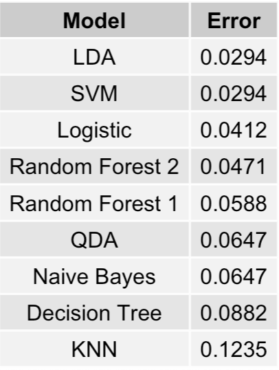
We have a tie between our Linear Discriminant Analysis (LDA) and Support Vector Machine (SVM), both having error rates of 2.94%. In other words, these two models correctly predict whether a breast cancer tumor is either malignant or benign 97.06% of the time (on the training data subset.) The logistic regression model comes in at 3rd place with an error rate of 4.12%, and I get served yet another humble pie. Although, in my defense, I did expect that the simpler linear models would perform best which is indeed the case.

The final thing to do is to fit the best models (LDA and SVM) on the entire data set instead of just the training subset and recalculate their error rates. Hopefully, one outperforms the other - ties are so anticlimactic don't you think?

								
####### Final Model Predictions #######
lda.final <- lda(diagnosis ~., Breast)
svm.final <- svm(diagnosis ~., Breast)
lda.final.err <- mean(predict(lda.final)$class != Breast$diagnosis)
svm.final.err <- mean(predict(svm.final) != Breast$diagnosis)
								
							

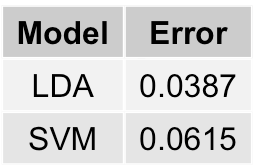
As shown above, Linear Discriminant Analysis is the best performing model, with a final comprehensive error rate of 3.87%. To wrap things up, I hope you are more convinced that breast cancer is a pressing issue, given its prevalence. I hope you agree that early detection is imperative in the fight against this disease, given how confident we can be in the diagnosis. Finally, I hope you think statistics is even cooler than you previously thought. Let's work together to spread the word! Enjoy the day.