Data Cleaning in R
Jan 20, 2024
Lecture Outline
- Introduction
- Tidyverse
- dplyr - transforming data frames
- lubridate - wrangling dates and times
- ggplot2 - visualizing data
- tidyr - cleaning data
- readr - importing data
- purrr - functional programming
- stringr - wrangling strings
- Final Exercises
- Appendix
Introduction
Welcome to another workshop. Today's topic is data cleaning, or wrangling. This can be defined as the act of transforming data in such a way
that is conducive to statistical analysis. For data to be clean, it should be without illegible elements, discrepencies, and corruption.
Corrupted data may have duplicated or incomplete values, they may have formatting issues or other flaws that may cause errors later on.
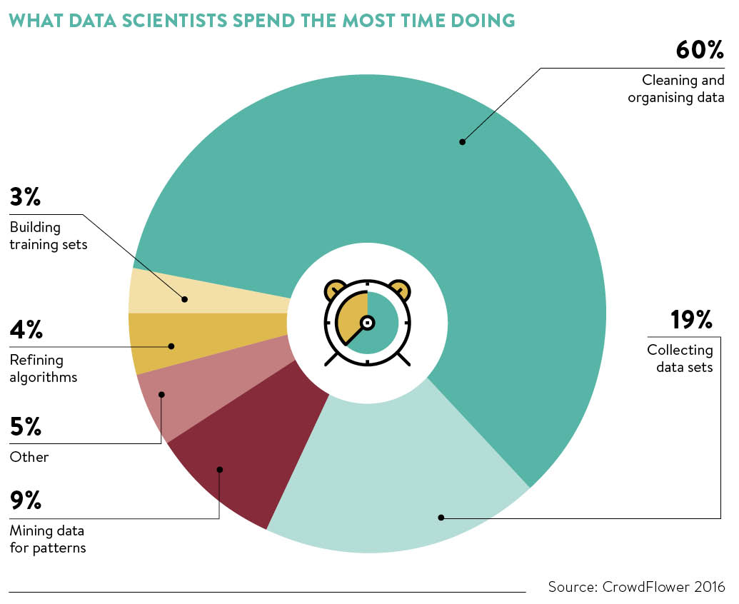
As shown in the plot above, data cleaning comprises most of the work data scientists engage in. For this reason, it is crucial for
data scientists to become experts in cleaning data. The purpose of this workshop is to introduce you to some of the most popular and widely used
packages for cleaning data.
Tidyverse
dplyr

Toy data set containing sales information for one week in a coffee shop. coffee_shop.tsv
- select() - select columns from your dataset
- filter(data, variable_name == "element") - filter out rows that meet your boolean criteria
- arrange() - arrange your column data in ascending or descending order
- join() - perform left, right, full, and inner joins in R
- mutate( ) - adds new variable or rewrites an old variable, within a data frame
- summarise( ) - aggregates variables using summary statistics (i.e mean, median)
- group_by( ) - groups a data frame by the levels of a specified variable
- |> - a pipeline operator that chains a sequence of calculations/tasks
- %>% - alternative notation for pipeline operation
#install.packages("tidyverse")
library(tidyverse)
coffee_shop <- read.table("~/Desktop/coffee_shop.tsv", header = TRUE)
View(coffee_shop)

filtered_coffee <- filter(coffee_shop, beverage == "latte")    						# filter()
filtered_coffee
filtered_coffee2 <- filter(coffee_shop, quantity < 40)
filtered_coffee2

grouped_coffee <- group_by(coffee_shop, date)                  						# group_by()
grouped_coffee

only_latte <- select(coffee_shop, quantity)                           					# select()
only_latte
all_but_date <- select(coffee_shop, beverage:price)
all_but_date

summarised_coffee <- summarize(coffee_shop, weekly_sales = sum(quantity * price))                  	# summarize()
summarised_coffee

mutated_coffee <- mutate(coffee_shop, sales = quantity * price)    		 			# mutate()
mutated_coffee

arranged_coffee <- arrange(mutated_coffee, sales)    # arrange()
arranged_coffee
arranged_coffee_desc <- arrange(mutated_coffee, desc(sales))
arranged_coffee_desc

only_mocha <- filter(mutated_coffee, beverage == "mocha")
only_mocha


######## Pipelines ########
pipe_ex <- 1:10
pipe_ex |> sum()
pipe_ex %>% sum()
pipe_ex |> mean()
pipe_ex |> order(decreasing = TRUE)

coffee_shop |>
  mutate(sales = quantity * price) |>
  filter(beverage == "latte")

coffee_shop |>
  mutate(sales = quantity * price) |>
  filter(beverage == "latte") |>
  summarise(weekly_latte_sales = sum(sales))
Checkpoint 1: General time to play around with the starwars data set
Challenge: Determine the BMI for each human. Hint: BMI = mass / (height/100)^2
lubridate

- year/month/day() - extracts components of an inputted date
- ymd() - converts string in YYYY-MM-DD format to date type
- as.Date() - converts string to date type
class(coffee_shop$date)
coffee_shop$date <- as.Date(coffee_shop$date)						# converting
coffee_shop$date <- ymd(coffee_shop$date)
class(coffee_shop$date)

year <- year(coffee_shop$date)								# extracting
year
month <- month(coffee_shop$date)
month
day <- day(coffee_shop$date)
day

my_day <- as.Date("2024-01-25")
my_day
next_month <- my_day + months(1) 							# arithmetic
next_month
next_year <- my_day + years(1)
next_year

start_date <- ymd("2024-01-01")
end_date <- ymd("2024-01-31")
days_between <- as.numeric(end_date - start_date)
days_between
ggplot2

- ggplot(data, aes()) - creates powerful plotting interface
- + geom_point() - scatter plot
- + geom_bar() - bar plot
- + geom_smooth() - LOESS
- + geom_hist() - histogram
- + annotate() - manually adds text to plot
- ... and many other functions that can be found here
ggplot(coffee_shop, aes(x = date, y = quantity)) + # scatter plot
geom_point()
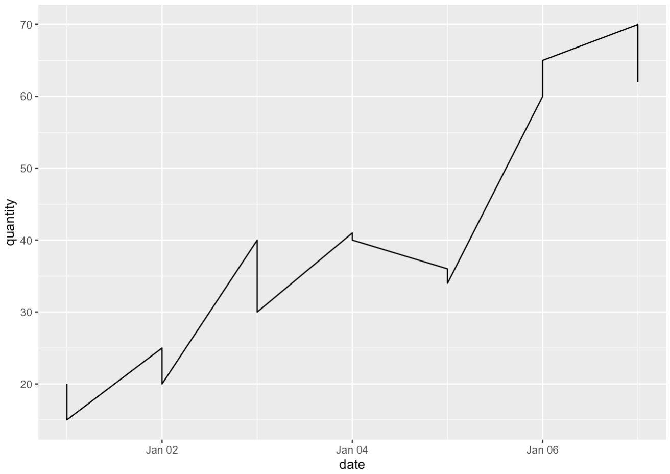
ggplot(coffee_shop, aes(x = date, y = quantity)) + # line graph
geom_line()
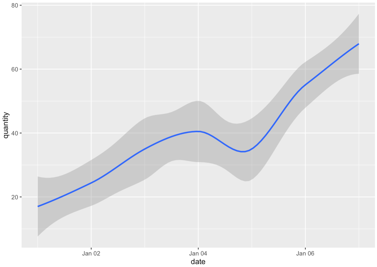
ggplot(coffee_shop, aes(x = date, y = quantity)) + # LOESS plot
geom_smooth()
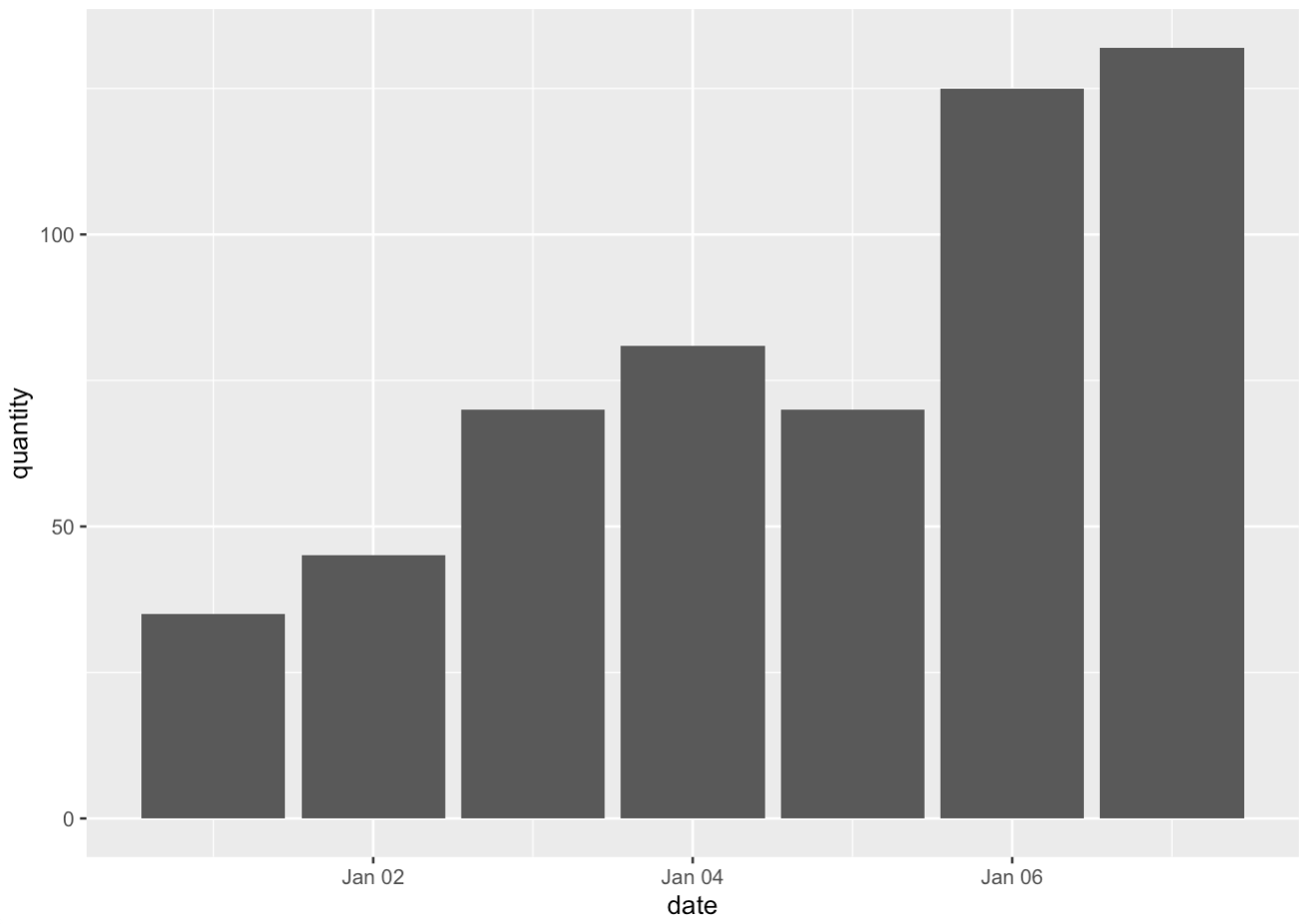
daily_sold <- coffee_shop |>
group_by(date) |>
summarise(quantity = sum(quantity))
View(daily_sold)
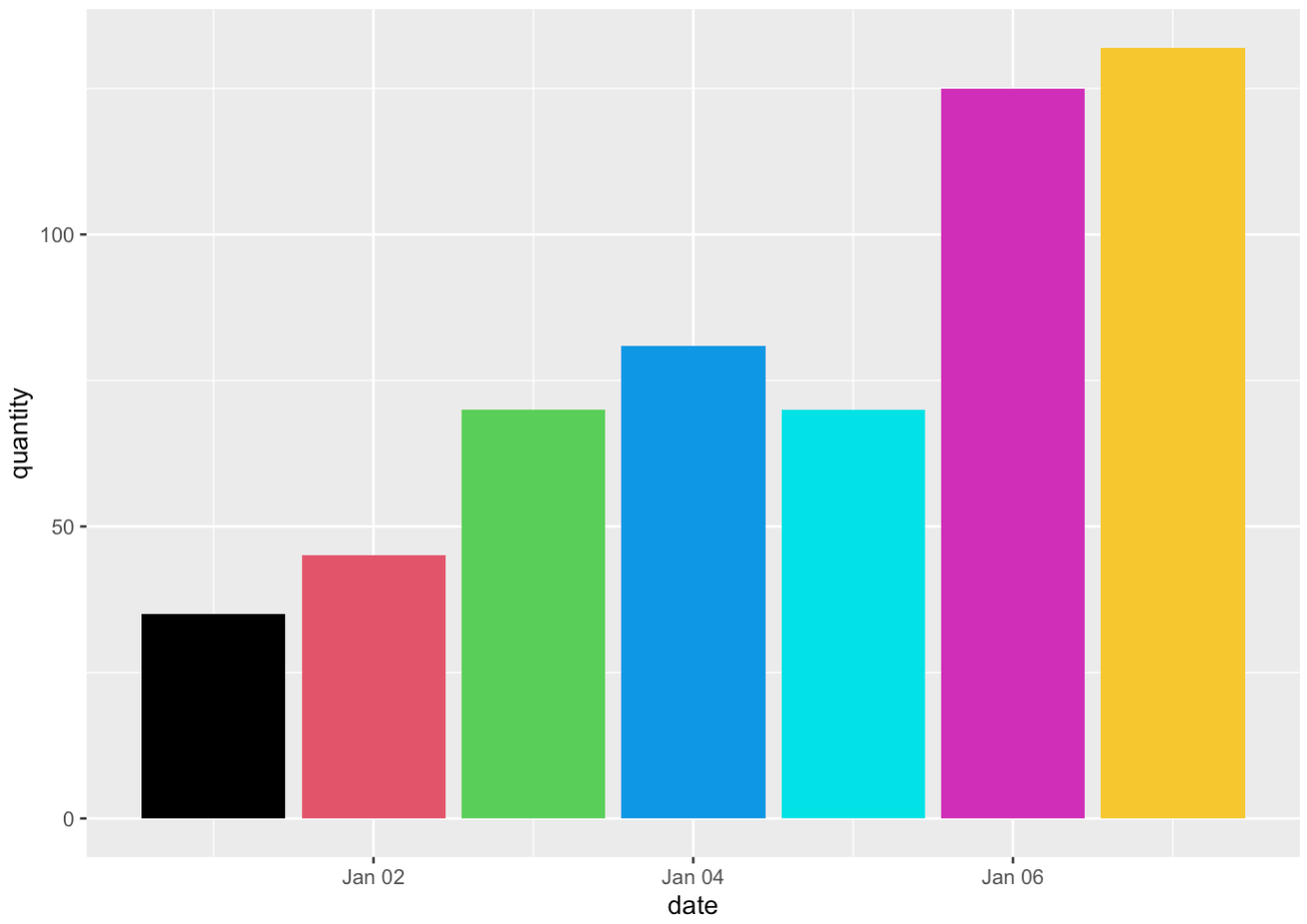
ggplot(daily_sold, aes(x = date, y = quantity)) + # bar plot
geom_bar(stat = "identity")
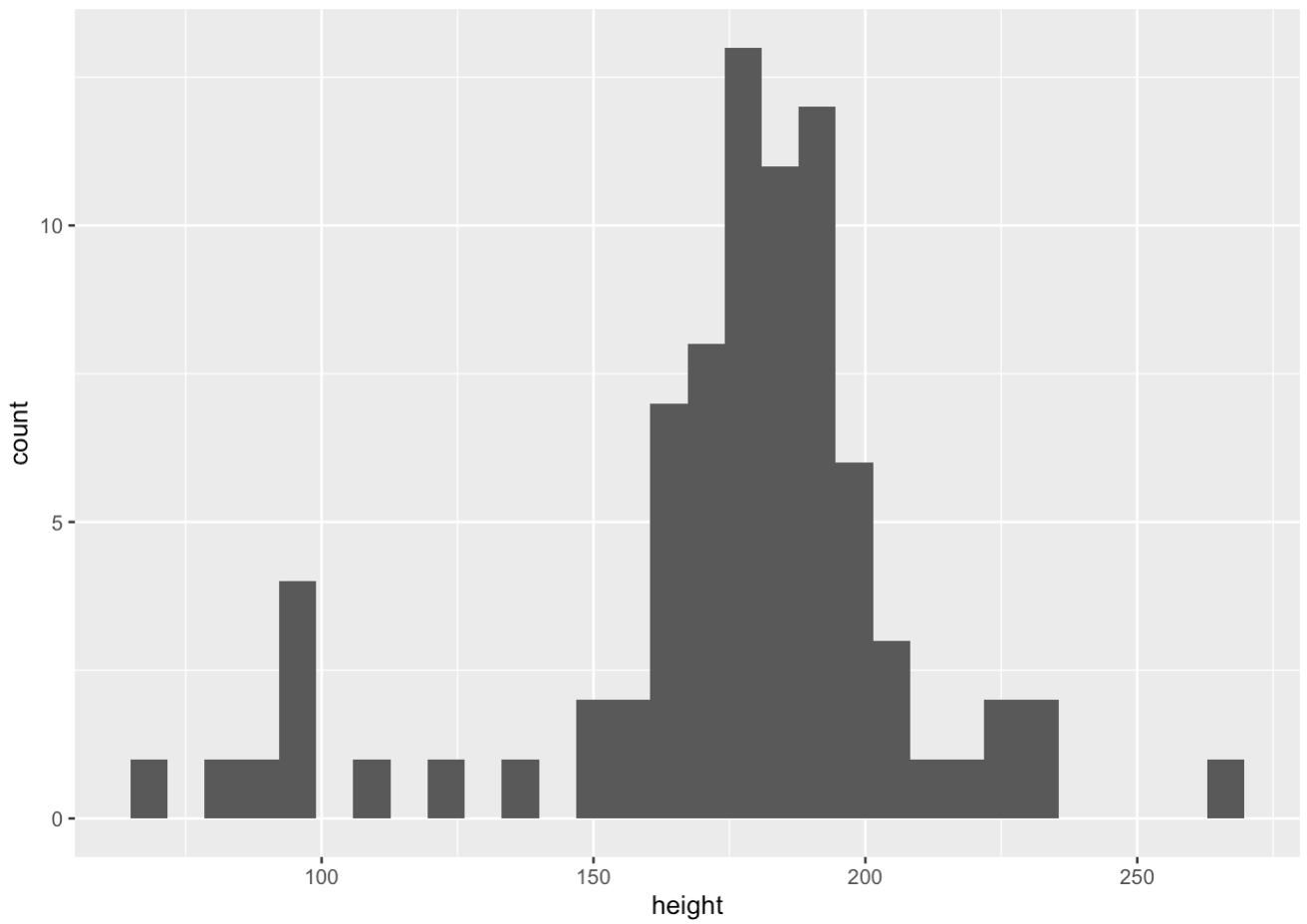
View(starwars)
ggplot(starwars, aes(height)) + # histogram
geom_histogram()
############# Customizing #############
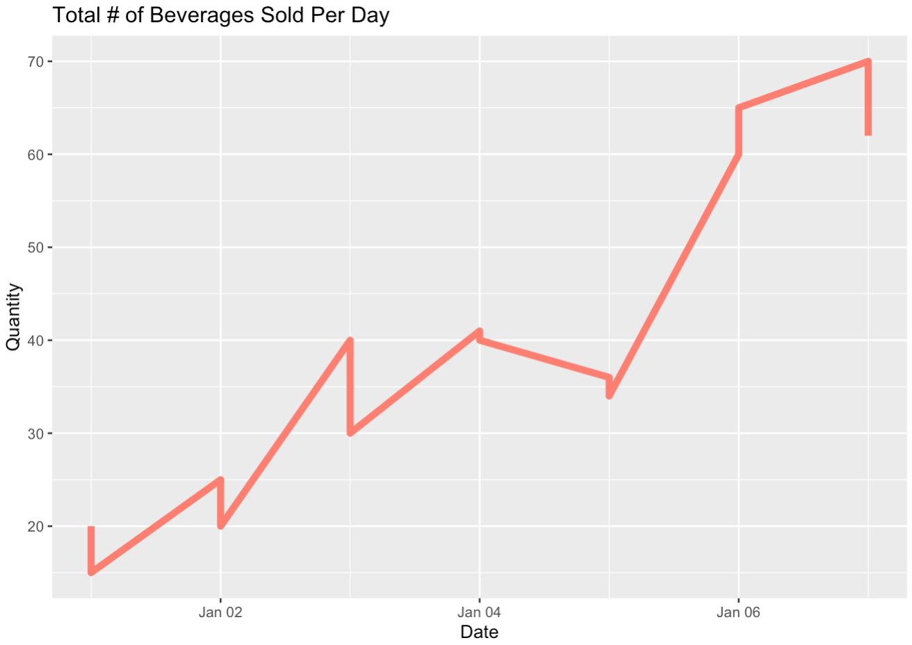
line_graph <- ggplot(coffee_shop, aes(x = date, y = quantity)) +
geom_line(col = "salmon", linewidth = 2) +
labs(x = "Date", y = "Quantity", title = "Total # of Beverages Sold Per Day")
line_graph
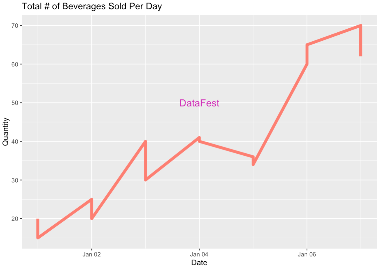
line_graph +
annotate(geom="text", x = ymd("2024-01-04"), y = 50, label = "DataFest", col = 6, cex = 5)
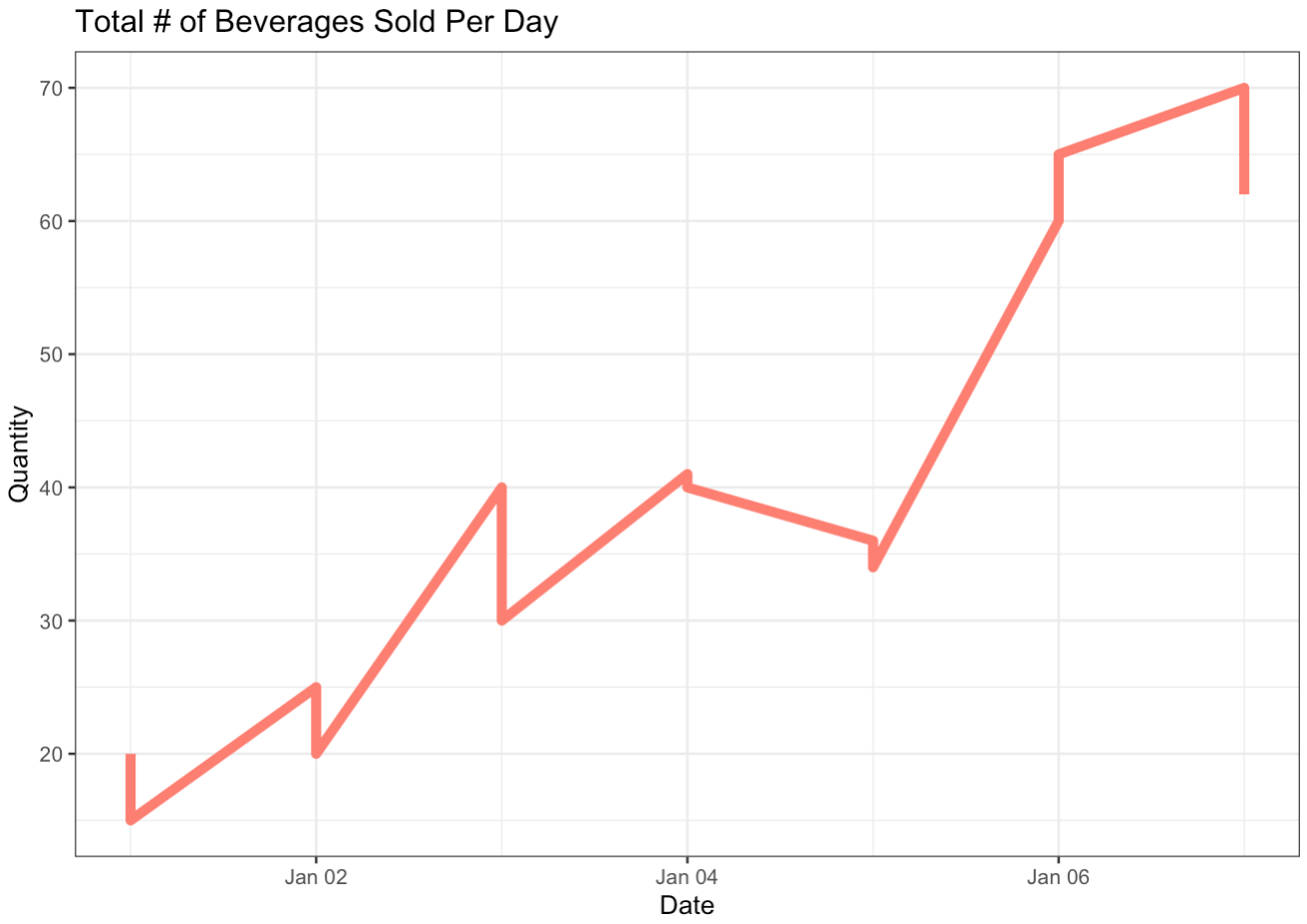
line_graph + theme_bw()
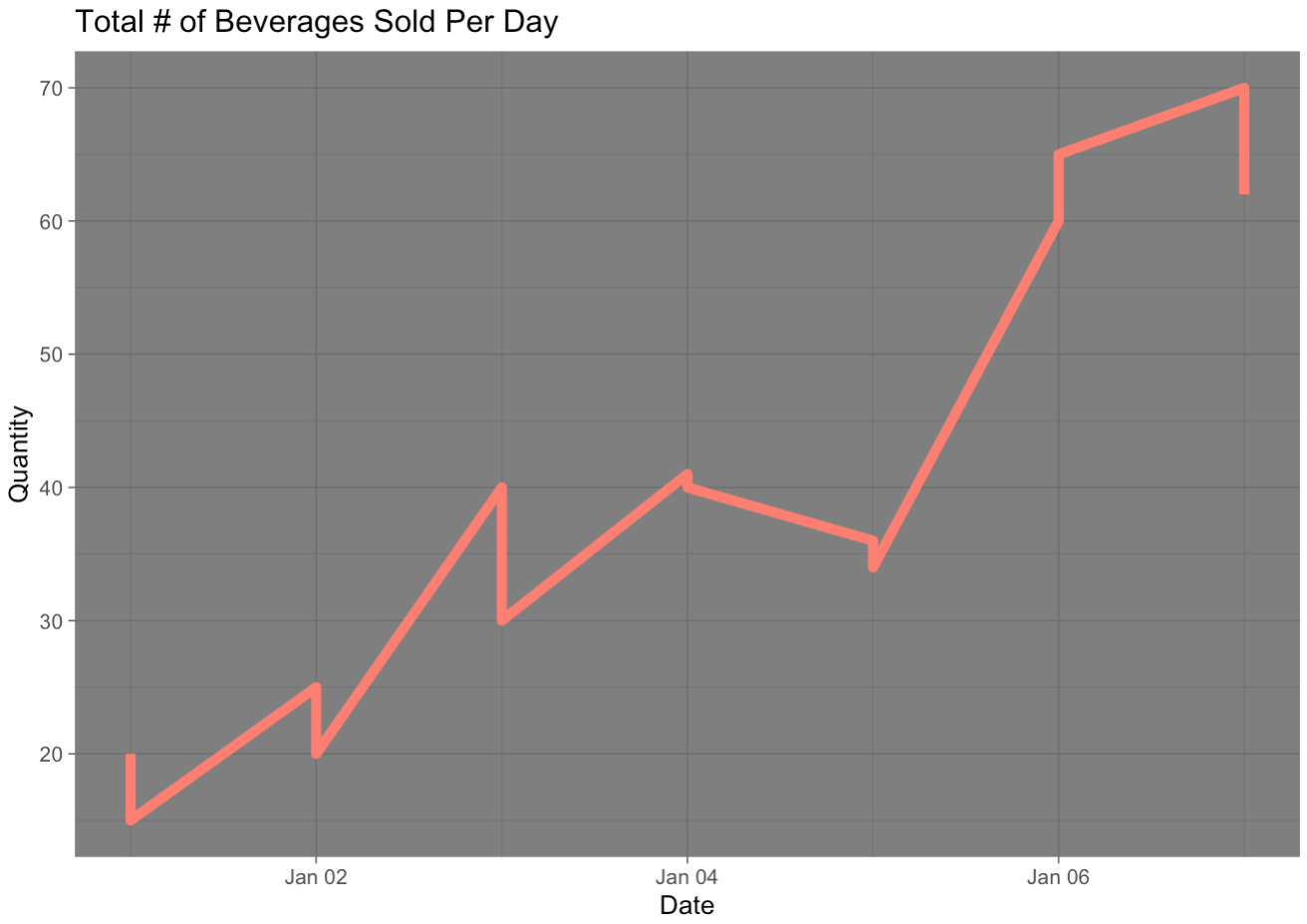
line_graph + theme_dark()
bar_plot <- ggplot(daily_sold, aes(x = date, y = quantity)) +
geom_bar(stat = "identity",
fill = 1:7)
bar_plot
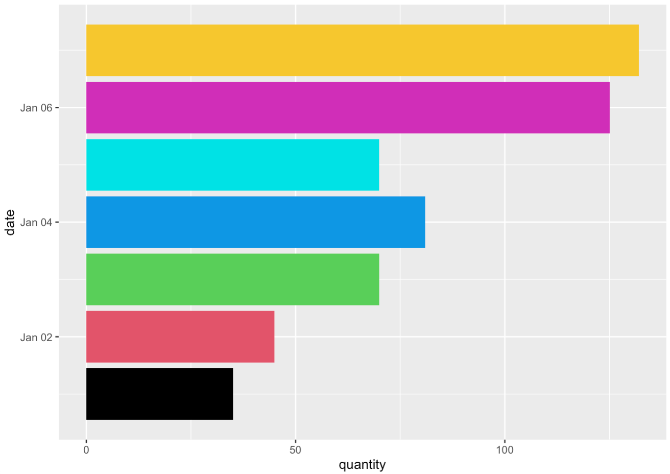
bar_plot + coord_flip()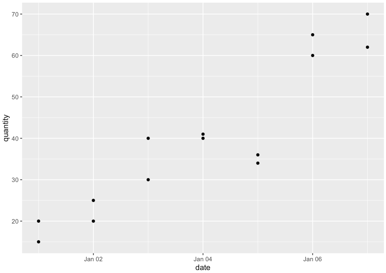
Checkpoint 2: Create a bar plot that showws total number of lattes sold each day
Challenge: Create a line graph showing the solution to the following system of equations: \begin{cases} y = 2x^{2} + 3x - 5 \\ y = sin(x) + \frac{1}{2}x \\ \end{cases}
tidyr

- gather() - converts df to long stretched out format, using column names as repeated elements
- spread() - this takes two columns and “spreads” them into multiple columns
- separate() - splits a single column into numerous columns - opposite of unite()
- unite() - combines two or more columns into one - opposite of separate()
- drop_na() - removes all rows containing an NA value
- replace_na() - replaces all rows containing an NA value, must input replacements as a list
################ gather() ################
gathered_df <- coffee_shop |>
  gather(Cols, Elements,
         beverage:price)
gathered_df


################ spread() ################
spread_df <- coffee_shop |>
                spread(beverage, quantity)
spread_df

spread_df |> drop_na()        									# drop_na()
spread_df |> replace_na(list(latte = 0, mocha = 0))         					# replace_na()


################ separate() ################
sep_df <- data.frame(Type = c("team.A", "team.B", "party.C", "crew.D", "party.E"))
sep_df

sep_df |>
  separate(Type, c("Group Type", "Letter"))

sep_df |>
  separate(Type, c(NA, "Letter"))


################ unite() ################
names_df <- data.frame(First = c("Harry", "James", "Stephen", "Michael", "Taylor"),
                       Last = c("Styles", "Bond", "Hawking", "Buble", "Swift"),
                       Age = c(29, 37, 76, 48, 34))
names_df

united_df <- names_df |>
  unite("Full Name", First, Last, sep = " ")
united_df

names_df |>
  unite("Full Name", Last, First, sep = ", ")

## How would we reverse unite?
united_df |>
  separate("Full Name", c("First", "Last"), sep = " ")
readr

- read_csv("path") - imports .csv file, input is the file path
- read_table() - whitespace-separated files
- col_types() - specifies desired column class types: character, factor, integer, etc
read_table("~/Desktop/coffee_shop.tsv")

read_table(
  "~/Desktop/Portfolio/dataCleaning/coffee_shop.tsv",
  col_types = cols(
      date      = col_date(format = ""),
      beverage  = col_factor(levels = c("latte", "mocha")),
      quantity  = col_integer(),
      price     = col_double()
  )
)
purrr

- map() - apply function to a list or atomic vector
- split() - divides vector into groups/tibbles
- \(x) - shorthand notation for defining a function (not specific to purrr package)
coffee_shop
coffee_shop |>                  						# split()
  split(coffee_shop$beverage)

## Quick Function Review ##
double_func1 <- function(x) x * 2
double_func2 <- \(x) x * 2
double_func1(15)
double_func2(15)

map(5, double_func1)
map(5, \(x) x * 2)        							# map()
5 |> map(\(x) x^2)

## What if we wanted to predict the # of lattes and mochas sold Jan 8th?
coffee_shop |>
  split(coffee_shop$beverage) |>
  map(\(df) lm(quantity ~ date, data = df)) |>
  map(\(model) predict(model, newdata = data.frame(date = ymd("2024-01-08"))))
stringr

- str_sub() - extract substrings
- str_length() - return string length
- str_split() - split string into list based on specified pattern
- str_count() - return occurance frequency of specified pattern
- str_detect() - return TRUE/FALSE depending on the existence of a specified pattern within string
- str_locate() - returns start/end indeces of specified pattern within string
- str_replace() - replaces pattern with specified alternative string
- select(ends_with("")) - enables more specific column selection
- str_to_lower()/str_to_upper() - converts the string into upper/lower case
a_string <- "Hello! I hope you're enjoying this workshop."
str_sub(a_string, start = 1, end = 5)
str_length(a_string)       # length
str_split(a_string, pattern = " ")
str_count(a_string, "o")
str_count(a_string, "[oab]")
str_detect(a_string, "joy")
str_locate(a_string, "you")
str_replace(a_string, "you", "we")
str_to_upper(a_string)

s <- str_split(a_string, pattern = " ")[[1]]
str_c(s, collapse = " ")

names(starwars)
starwars |>
  select(ends_with("color"))
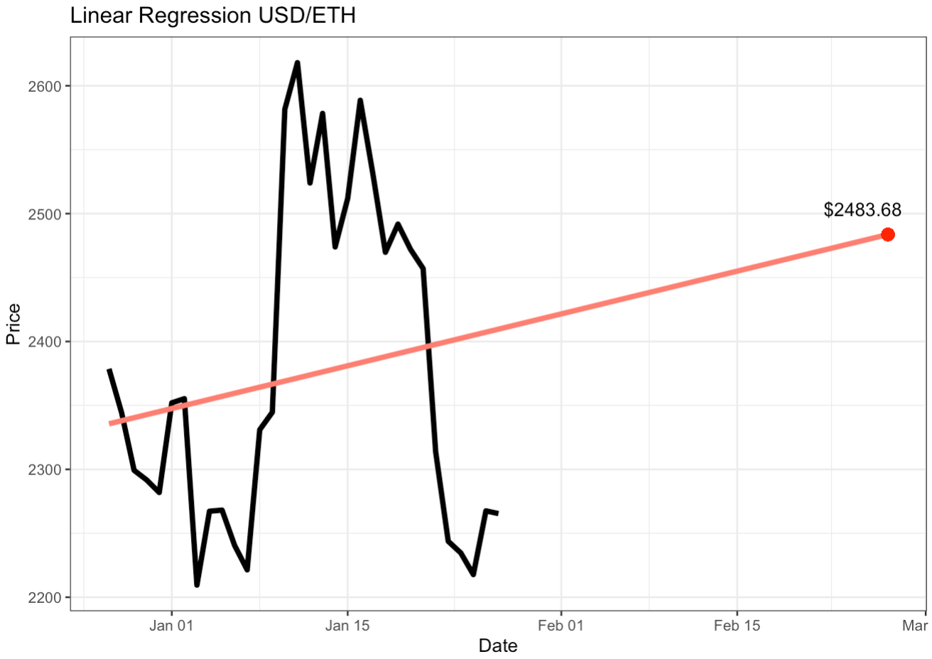
Final Exercise
- Download the current market data for Ethereum from this website: Investing.com
- Read in the file
- Clean the data, specifically:
- Convert Date column to date type
- Transform the Vol. column to the correct numeric values - look out for 'K' and 'M' units
- Transform the Change % to numeric type
- Predict the USD/ETH price for next month
- Plot the results using ggplot
Appendix
Exercise Solutions
- Star Wars BMI
- Lattes Sold Each Day
- Plotting Solutions to a System of Equations
- Final Exercise
starwars |>
  filter(species == "Human") |>
  mutate(bmi = mass / (height / 100) ^ 2) |>
select(name, bmi)latte_by_day <- coffee_shop |>
filter(beverage == "latte")
ggplot(latte_by_day, aes(x = date, y = quantity)) +
geom_bar(stat = "identity", fill = 1:7, alpha = 0.7) +
labs(x = "Day", y = "Lattes Sold", title = "Total # of Lattes Sold Per Day") +
theme_bw()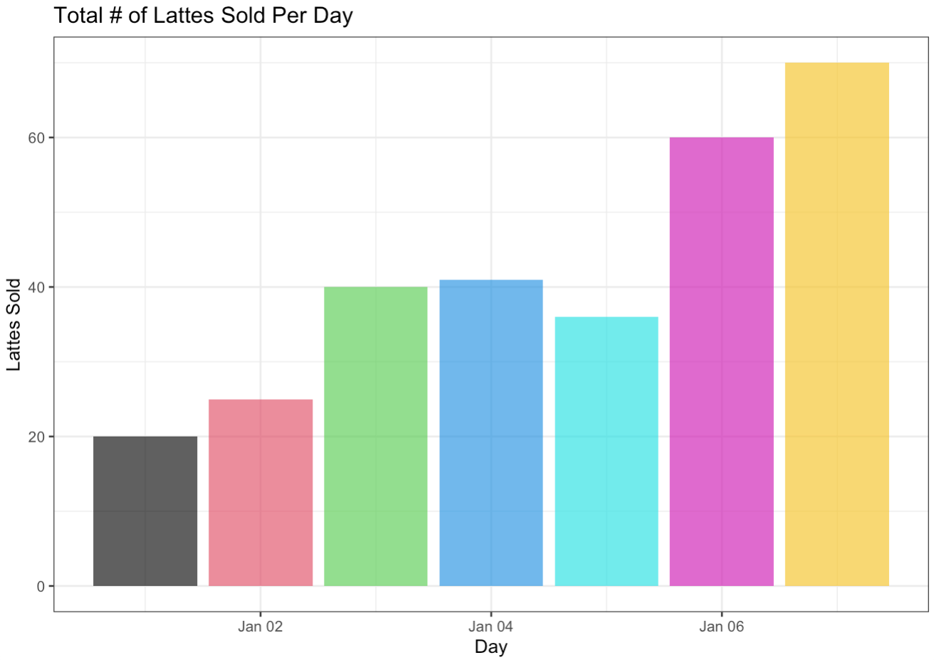
x = seq(-10, 10, 0.1)
y1 = 2*x^2 + 3*x - 5
y2 = sin(x) + x/2
sys_eq_df <- data.frame(x, y1, y2)
ysol <- y2[which(round(y1, 1) == round(y2, 1))]
xsol <- x[which(round(y1, 1) == round(y2, 1))]

ggplot(sys_eq_df, aes(x1)) +
  geom_line(aes(y = y1, col = "salmon"), linewidth = 1) +
  geom_line(aes(y = y2, col = "skyblue"), linewidth = 1) +
  theme_bw() +
  ylim(-10, 10) +
  labs(x = "x", y = "y") +
  scale_color_discrete(name = "Lines", labels = c("y1", "y2")) +
  geom_point(x = xsol[1], y = ysol[1], col = "red", cex = 3) +
  geom_point(x = xsol[2], y = ysol[2], col = "red", cex = 3) +
  annotate(geom="text", x = 3.3, y = 0.3, label="(1.2, 1.53)") +
  annotate(geom="text", x = -4.1, y = -3, label="(-2.2, -1.91)")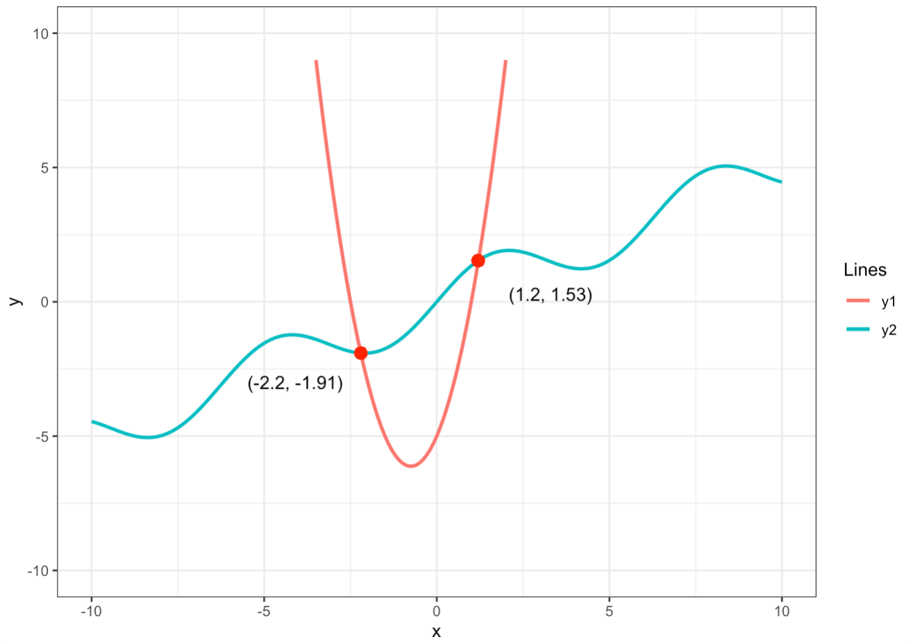
### Step 1: Read in data
eth_df <- read_csv("~/Desktop/eth.csv",
                   col_types = cols(Date = col_date(format = "%m/%d/%Y"))
                   )

### Step 2: Clean data
k <- str_detect(eth_df$Vol., "K")
m <- str_detect(eth_df$Vol., "M")

eth_df$Vol.[k] <- str_sub(eth_df$Vol.[k], start = 1, end = 6) |>
                  as.numeric() |>
                  map(\(x) x * 1000)

eth_df$Vol.[m] <- str_sub(eth_df$Vol.[m], start = 1, end = 4) |>
                  as.numeric() |>
                  map(\(x) x * 1000000)

eth_df$`Change %` <- eth_df$`Change %` |>
                     str_replace("%", "") |>
                     as.numeric()

### Step 3: Fit model and predict price
lm <- lm(Price ~ Date, data = eth_df)
days <- seq(ymd('2023-12-27'), ymd('2024-02-27'), by='1 day')
pred <- predict(lm, newdata = data.frame(Date = days))

### Step 4: Plot
eth_df[33:63, ] <- NA
ggplot(eth_df, aes(Date, Price)) +
  geom_line(linewidth = 1.5) +
  geom_line(aes(x = days, y = pred), col = "salmon", linewidth = 1.5) +
  theme_bw() +
  ggtitle("Linear Regression USD/ETH") +
  annotate(geom = "text", x = ymd('2024-02-25'), y = pred[63] + 20, label = "$2483.68") +
  geom_point(x = ymd('2024-02-27'), y = pred[63], col = "red", cex = 3)