An Ethereum Regression Analysis
December 14, 2023
(March 10, 2024 Update) A less detailed, but more statistically rigourous forcast modeling analysis can be found on my blog here.
The primary purpose of this article is to predict the price of the blockchain currency, Ethereum (ETH). A secondary purpose is to teach simple, modern, and
effective regression modeling methods. I intend to keep things simple and straightforward.
Before we jump in, I'd be remise not to remind you that Ethereum is infamous for being extremely volatile. Like farting in a hurricane, it could go anywhere at anytime.
This makes regression, even with all the bells and whistles of statistics, a risky process. Please process claims made in this analysis with a moderate degree of skepticism.
The Data
The data we will be using for today's analysis was downloaded from Investing.com.
The data set is historical ETH price data from July 1, 2017 to December 13, 2023. This makes for 2, 356 observations to model.
We will focus on two variables: Date and Price. Date acts as our predictor, with Price as our response.
Some data cleaning was performed to make for clear, numeric values. As noted earlier,
I want to keep things simple and straightforward. There's nothing more straightforward than a straight line, so we start by fitting a
linear function to out training data:
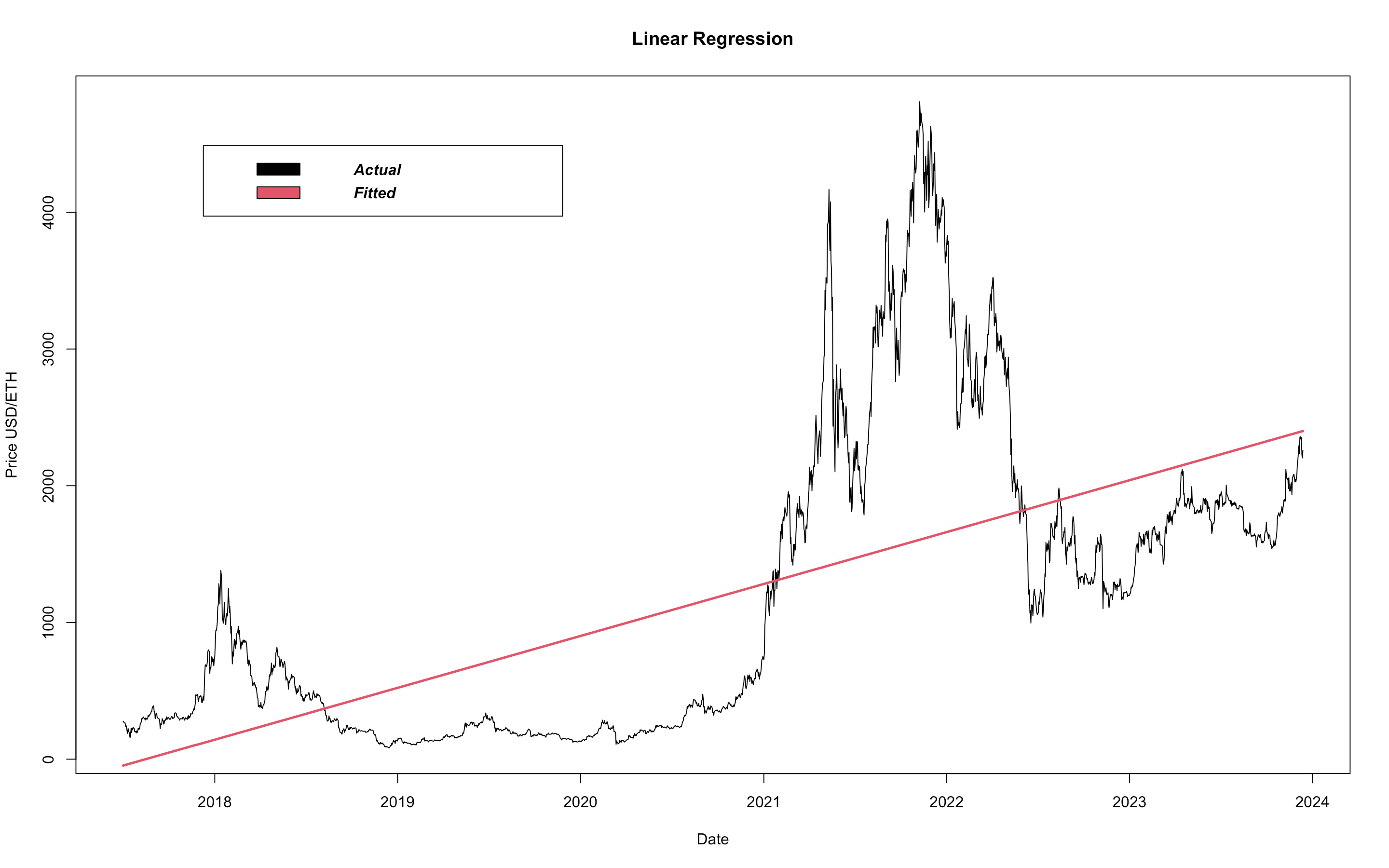
Straight lines are useful in that they are robust and smooth, but, linear models do not allow for a flexible fit. A model's flexibility refers its ability to 'bend' to the data. A highly flexible model is a curvy model, enabling the model to touch more data points. So, to increase a model's flexibility we need to increase its curvature and we do that my increasing the dimensionality of the function. A linear model has dimensionality of 1. Let's compare this to a model with dimensionality of 2, better known as a quadratic model:
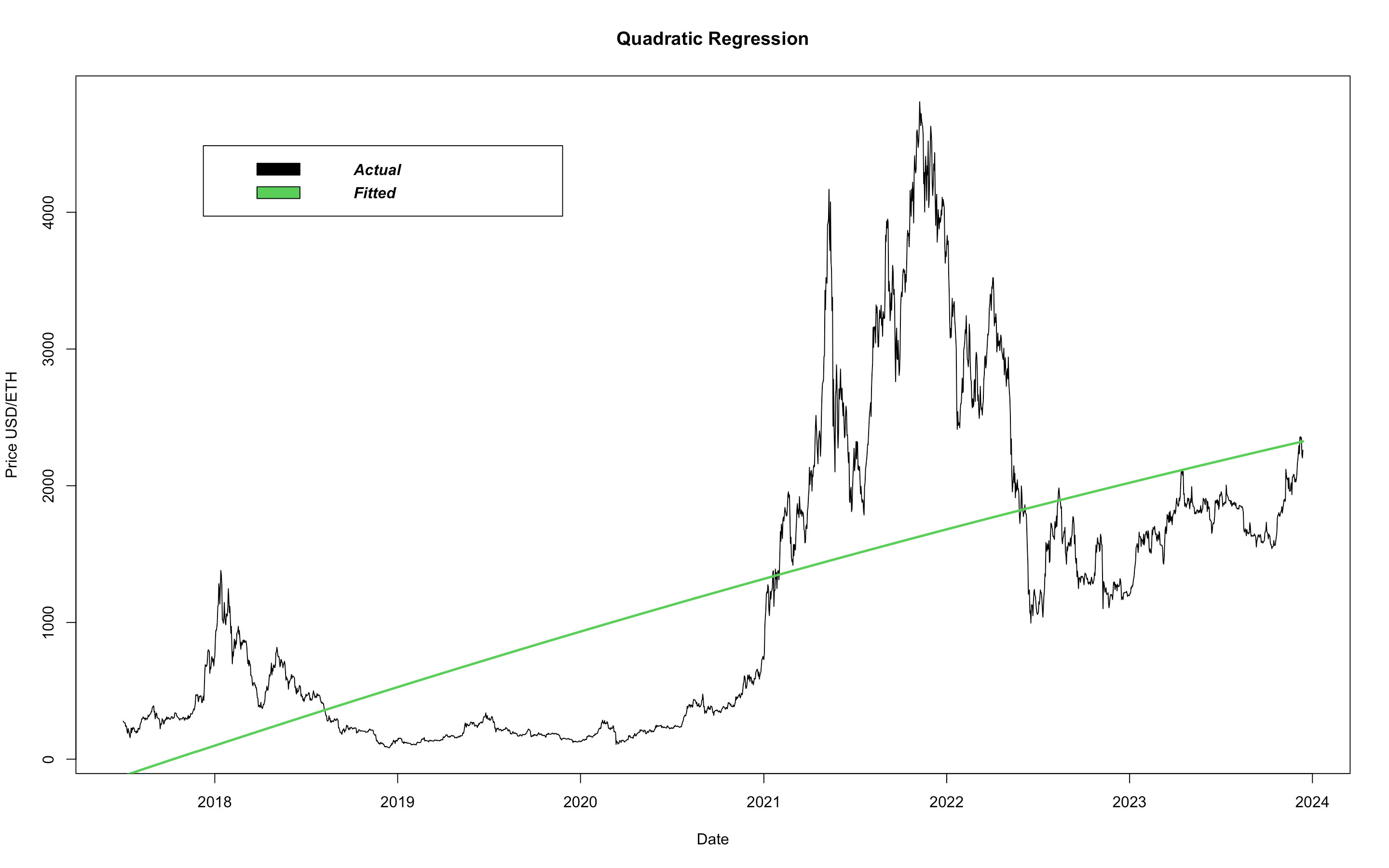
It's difficult to see a difference between the linear model and the quadratic model. Note the concavity, this model is barely curving downwards, signifying the maturity of the currency. Peaks get less prominent as equities mature. As ETH has matured, volume has increased and, as a result, volatility has decreased. We continue by looking at a 3rd degree polynomial fit, a cubic model:
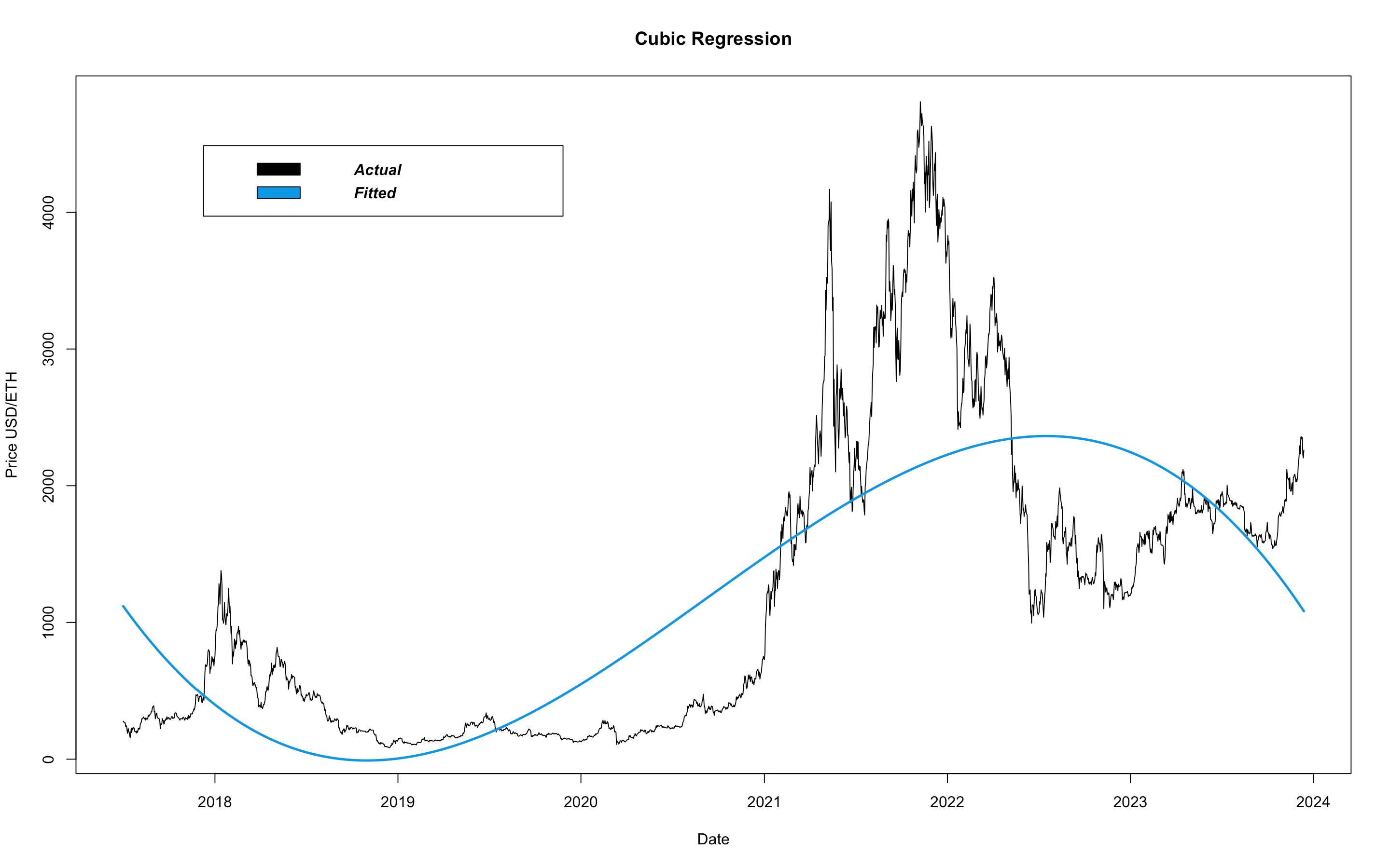
From this, it is much more clear that increasing dimensionality results in a more flexible and curvy fit. This model tracks more closely to the observed data than the previous models. However, if we were to use this model to predict into the future, prices would decrease at an increasing rate, eventually surpassing a $0 and moving to negative values. This, of course, poses an issue. So the optimal regression model finds the correct balance between flexibility and predictability. We can continue to increase the dimensionality of our polynomials so that the models align more and more closely to the data, but then the predictability will become less reliable. So let's move away from polynomials and look at a logarithimic model:
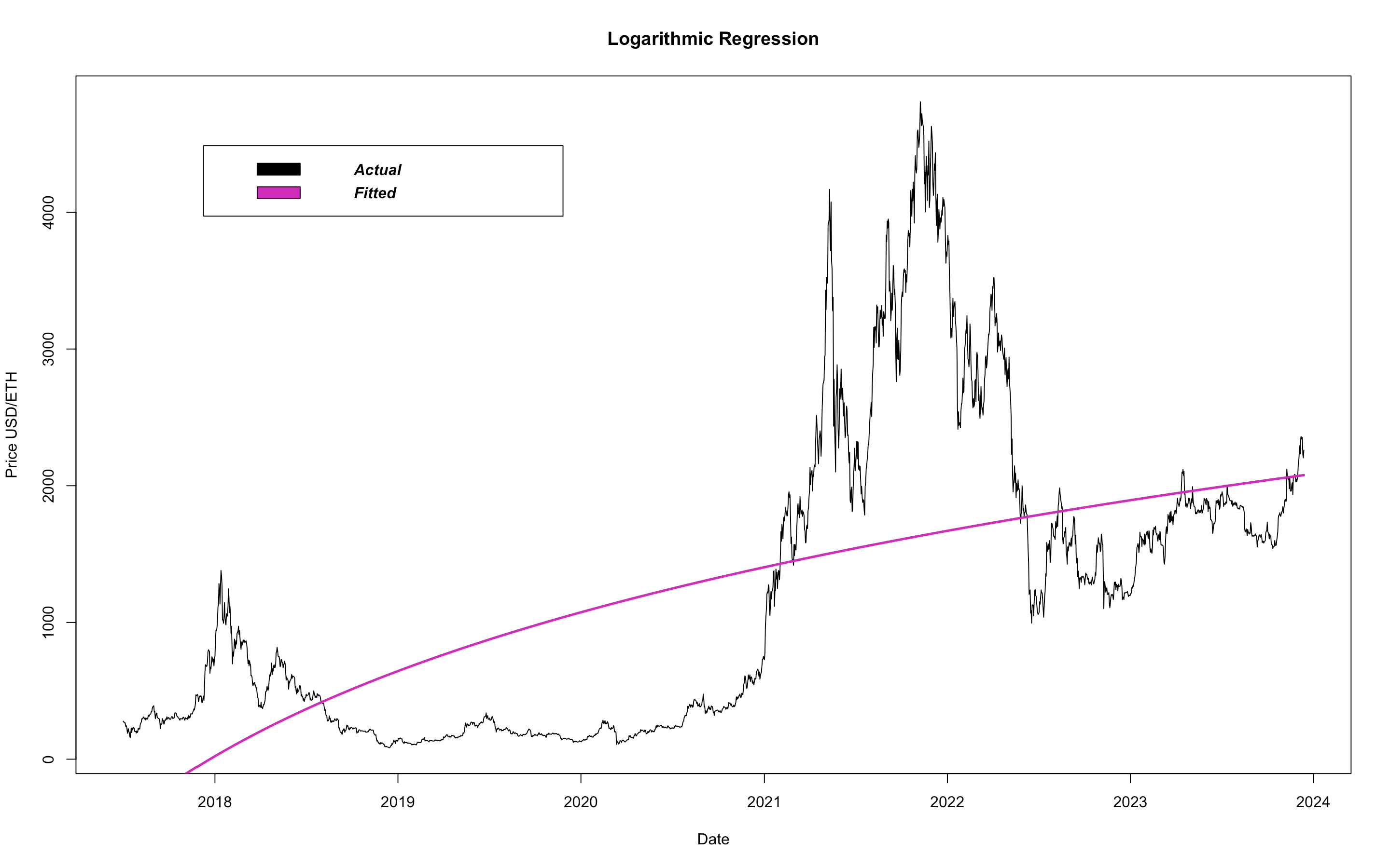
As you can see, a logarithimic model does well to proivde a flexible fit while preserving its integrity. Logarithms are monotonic functions, and so this model will never predict negative price values. Further, it predicts the price will always increase, but will do so at a decreasing rate. This aligns with algorithimic trading theory. To keep going just a little further, since we just fit a logarithm, let's compare it with its inverse, the exponential:
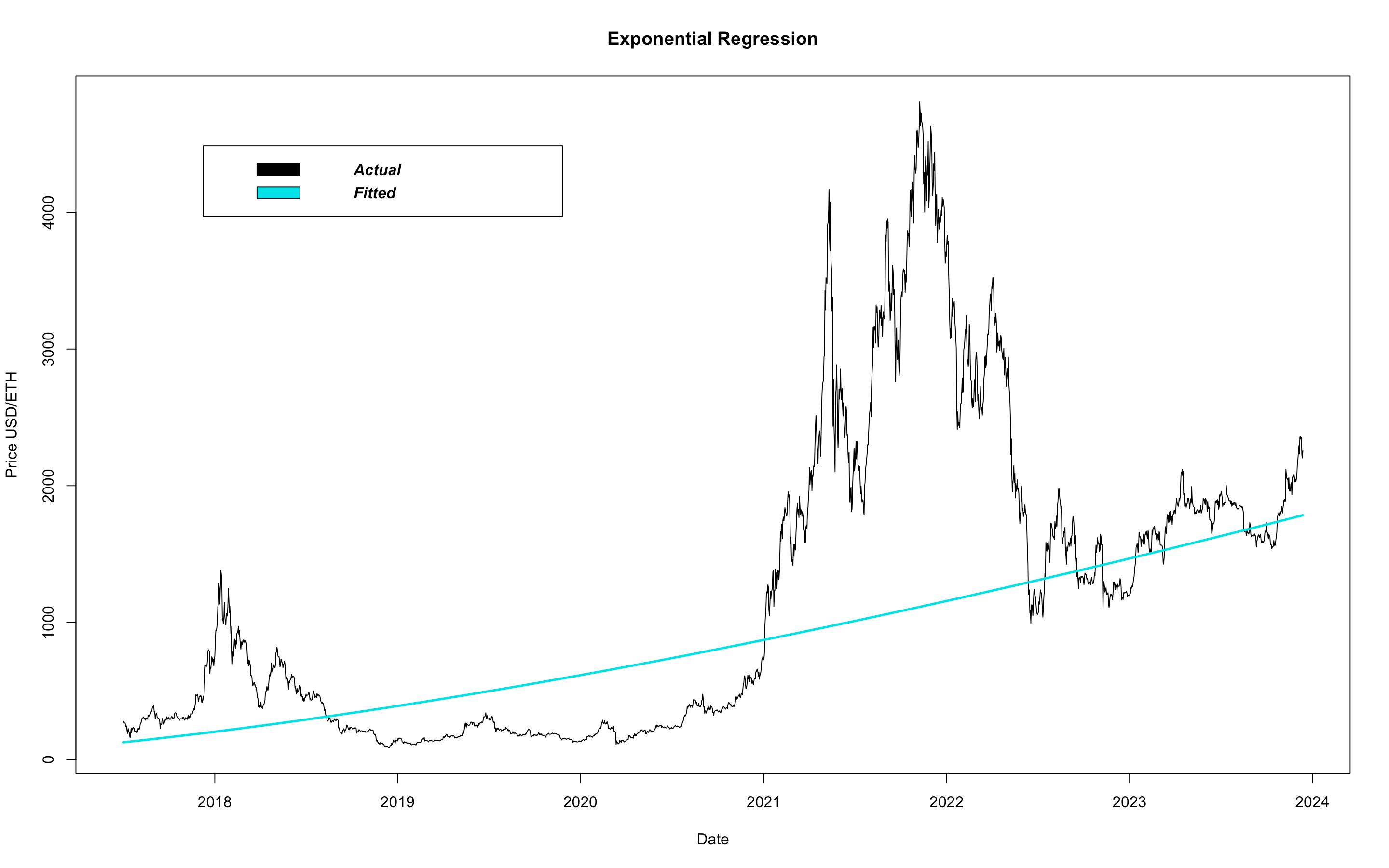
This model does well to provide the right amount of flexibility, but it assumes ETH price will increase at an increasing rate. As much as we'd like to believe this,
it is not how equities behave and so we must reject this assumption.
As a quick side note, we can fit a
Generalized Additive Model (GAM)
to leverage the power of smoothing splines and produce an exceedingly flexible model.
As you'll see, this does really well at fitting the data.
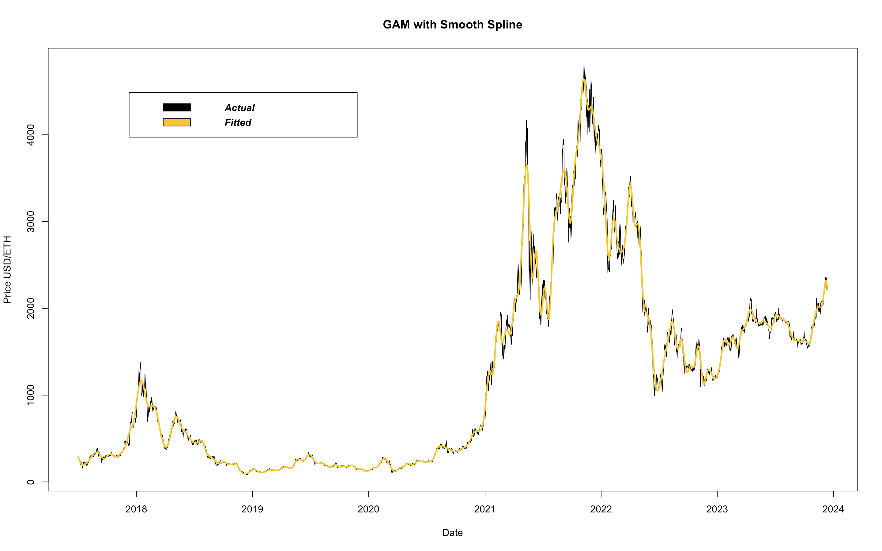
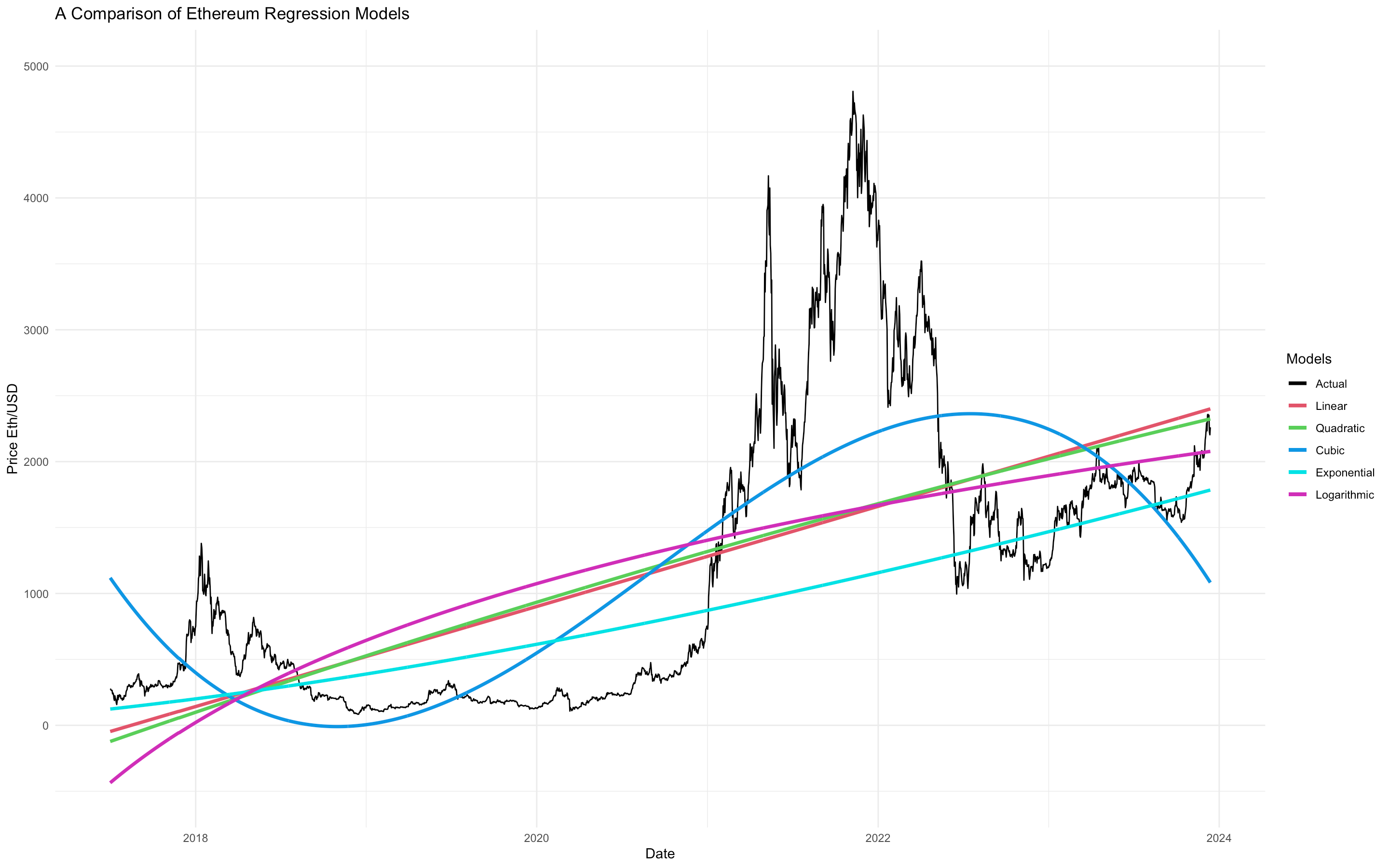
A nearly a perfect fit. However, as discussed earlier, because this model is so flexibile, it will perform poorly when asked to predict into the future. To show this, here are all the models on one plot. Note, the more flexible models perform the worst when predicting future prices.
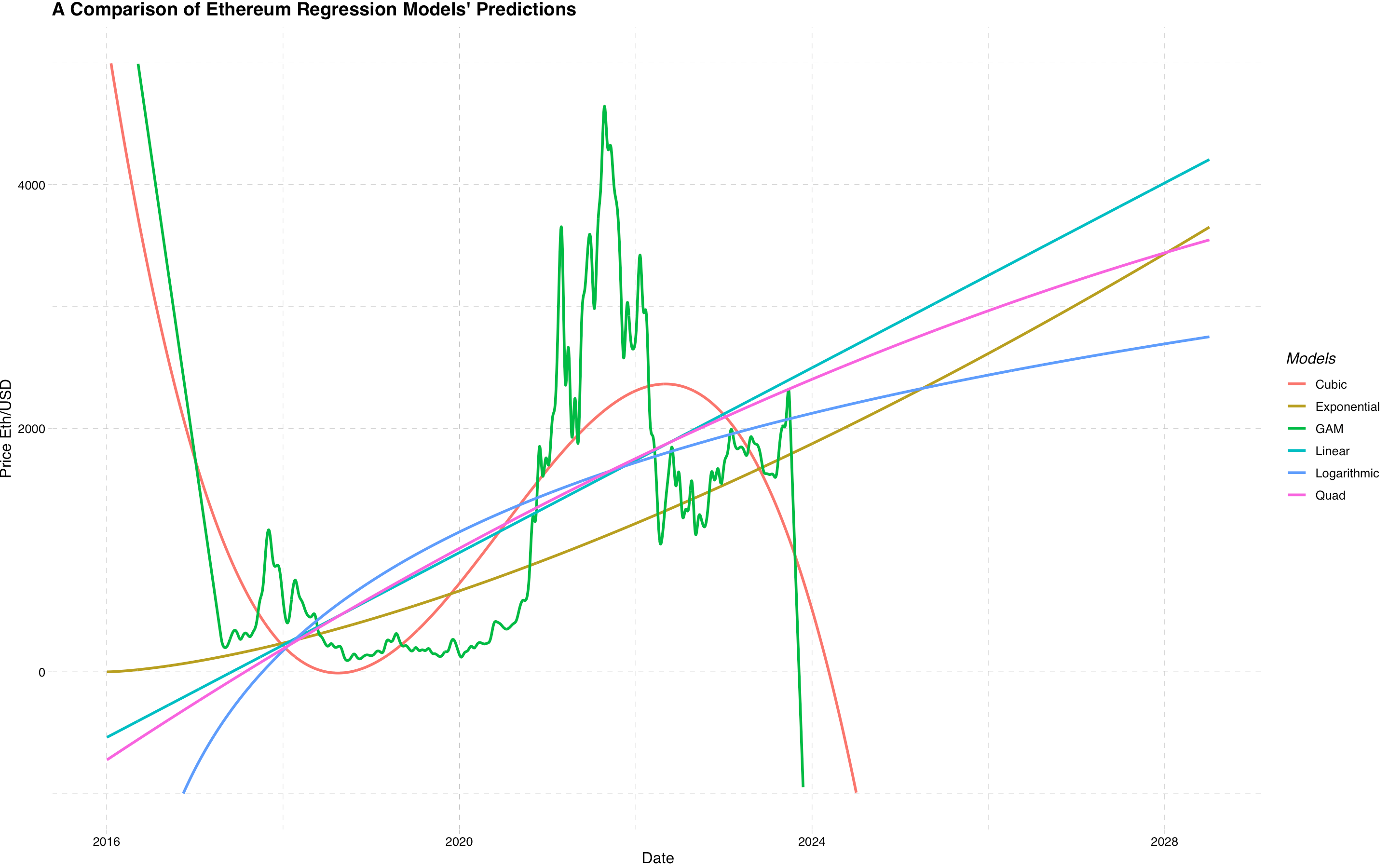
To determine the best model analytically, we must first take a quick tangent to discuss a popular metric called Mean Sqaured Error (MSE) . Simply put, MSE tests how inaccurate a model is. Eye-balling graphs can only get us so far, so we need a reliable metric to quantify inaccuracy - enter MSE. We will begin by fitting a few models to our training set - a set that contains the avgerage daily price for the first 80% of days. We refer to the remaining 20% of days as the test set. To compute the MSE of a model, we ask our models to predict the remaining 20% of data and then compare that prediction to the actual observed data in the test set. This is the metric we'll use to quantify how inaccurate our models are. Considering the table below, the model with the lowest MSE is the one that best fits the test data.
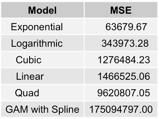
The best model is revealed as a Logarithmic Regression model. Here it is again:
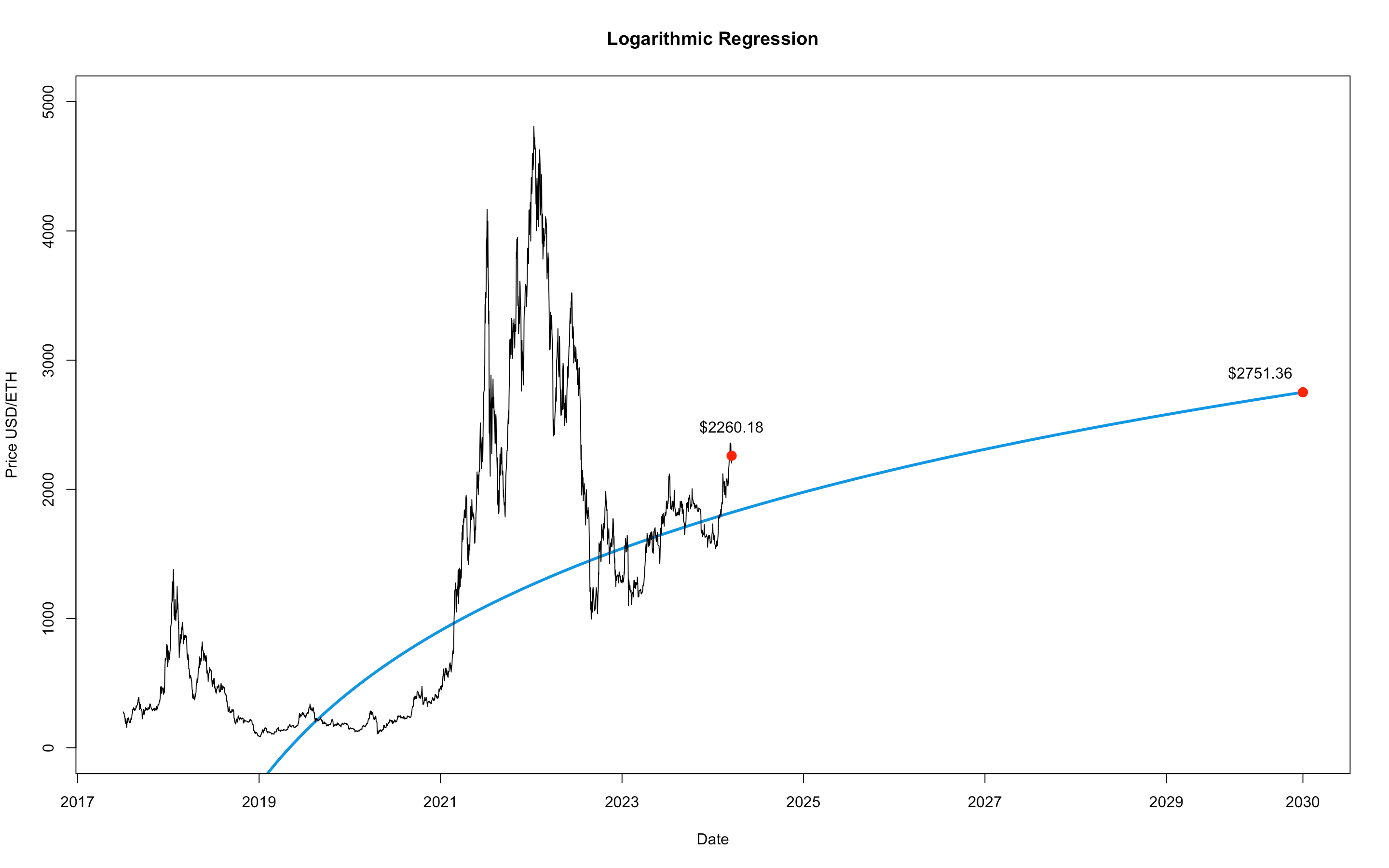
So, according to our optimal model, Ethereum will be priced at $2751,36 on New Year's Day of the year 2030. Invest responsibly.