An Artificial Neural Network Approach to Identifying Diabetes Risk Status

December 8, 2023

Today's article is one meant to educate about neural networks and their inner workings. I'll walk through the process of coding a neural network explaining the relevant math and concepts behind it, including powerful ideas such as gradient descent and forward/backward propagation. Neural networks are a complex topic so to help explain and understand the ideas, we will work through a classification problem. Our task will be to classify peoples' risk of developing type 2 diabetes.

---

A Metaphor on Sorting Big Data

---

To get a better idea of the complexity this requires, let's imagine skittles and a strainer. You have a MASSIVE bag containing hundreds of thousands of skittles and only one strainer with only three holes in it - the idea being we need to sort these skittles into three different groups. You begin to pour your bag of skittles into the strainer to separate them. Almost immediately, you notice issues with this process because the strainer is too constrictive and can't handle so many skittles. Some skittles get sorted through, but only few at a time. While you are waiting for your skittles to slowly move through, you see another strainer. This one has ten holes in it and a brilliant idea pops into your head - you place the strainer with ten holes atop the strainer with three holes and continue to pour the skittles into this stack of now two strainers. Note, we can say this system of strainers has two layers. Your idea works! You notice the skittles are sorting through the system at a faster rate than when you had just the one strainer. So, to further expedite this process and increase the power of your system, you go out to buy more strainers with more holes and add them as additional layers to your system. This is one method to handle extremely large data sets, or big data.

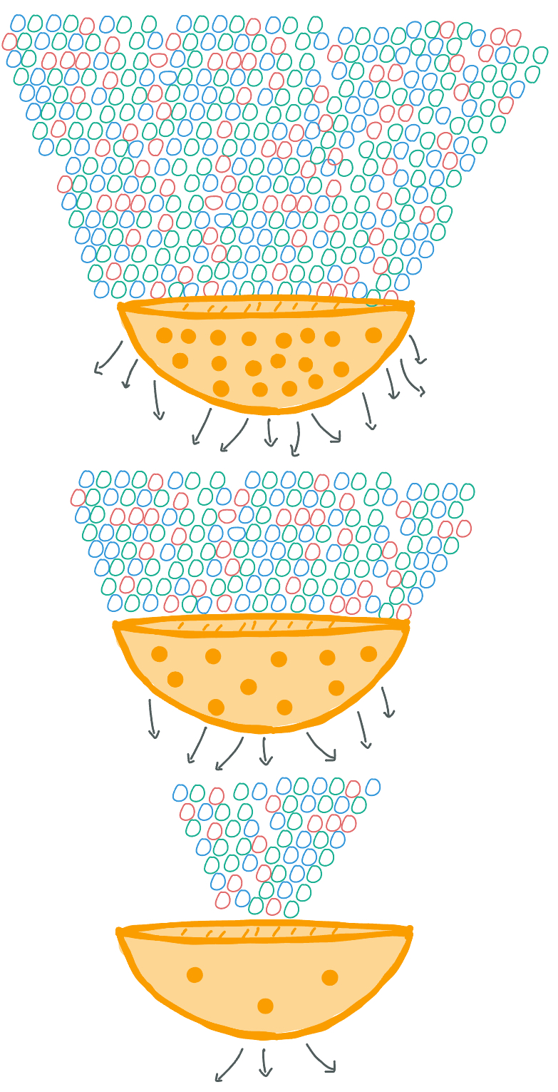
Figure 1. A diagram to help visualize a popular sorting method often implemented to handle big data.

---

The Data

---

Today's task is to identify a person's risk of developing type 2 diabetes, given some information about their biology and lifestyle. As of 2019, 37.3 million Americans had been diagnosed with diabetes and 96 million had prediabetes - defined as having high risk of developing type 2 diabetes ¹. Type 2 diabetes is a chronic disease that describes the body's difficulty in either producing or properly utilizing insulin. Insulin is produced and secreted by the pancreas to help break down glucose (i.e. sugar) in the foods you eat. For this reason, people who have diabetes are much more likely to have abnormal levels of glucose in their bloodstream - this metric is commonly referred to as blood sugar levels. If neglected, extremely high or extremely low blood sugar levels can lead to a multitude of health complications such as heart disease, kidney disease, hearing loss, and cataracts, to name a few ². Type 2 diabetes is preventable and treatable. With proper nutrition, exercise, and lifestyle habits, people with type 2 diabetes can function at high levels with minimal effects on their daily lives. Before we can implement corrective regimens, however, we must first be able to identify one's diabetes risk status. The neural network we will build today, trained using robust and reliable data, will help us do just that.

The data set we will be using has been generously provided by the Center for Disease Control and Prevention (CDC) as a part of their annual behavioral survey of Americans. In this survey, people are asked questions about their biological health factors and lifestyle habits. Specifically, we have 253, 680 people and 21 variables for each person. This makes for over 5 million values for our network to track. Furthermore, to add to the complexity, many of these variables have two or more levels - meaning they have two or more possible values they can equal. For example, General Health ranges from 1-5, whereas Mental Health ranges from 1-30. All the variables are either numeric, ordinal, or binary, and they all eventually need to morph into a single output value: diabetes risk status. We will define diabetes risk status to hold one of two different values: low risk and high risk.
The variables in our data are as follows:

---

Artificial Neural Networks

---

An artificial neural network is a classification algorithm setup in such a way as to artificially mimic the human brain. A brain's neural network is a web of interconnected neurons (aka nodes) that are activated only when deemed relevant to particular information. Nodes are connected by message pathways; these pathways will strengthen or weaken depending on their relevance. As a simple example, let's say node 1 is good at identifying animals and node 2 is good at identifying ice cream flavors. If you were to sit down and watch The Lion King, node 1 will be much more active than node 2. You can get a sense of how complex this web becomes when you consider all the animals that exist and the often subtle differences between them. It is so complex, in fact, there approximately 100 billion neurons in the human brain³.

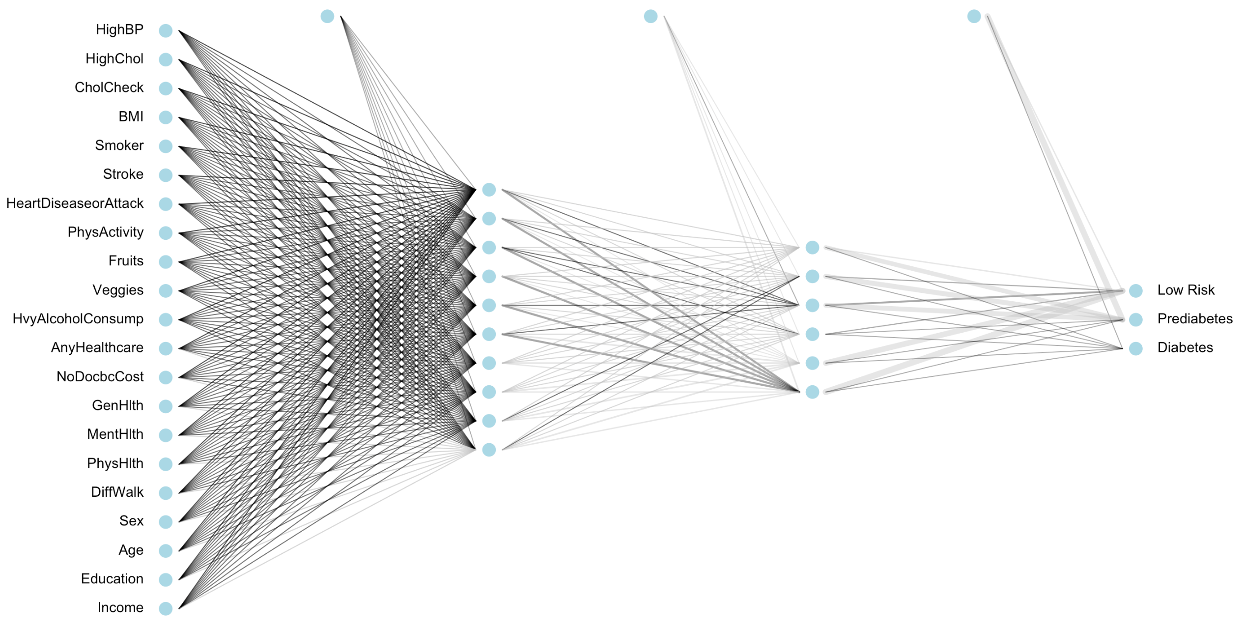
In our diabetes example, to sort 253, 680 observations we will code a system with three layers. The first layer is called the input layer and will take in all 21 variables for each individual person. The second layer is considered to be a hidden layer. The final layer is the output layer and will sort the last hidden layer into 2 groups (diabetes risk status). Any layer that is between the input and output layers are considered hidden layers. If a neural network has many hidden layers, it is considered to be a deep neural network.

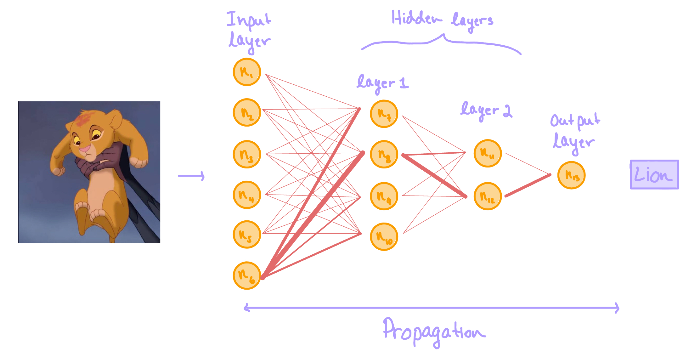
Figure 2. A diagram portraying the general structure of an artificial neural network. The orange circles are nodes which are analogous to neurons in the brain. The red-orange lines represent the information pathways between nodes. The thickness of each line symbolizes the relevance of the connection - as thickness increases, relevance increases.

Consider the neural network diagram above. The task of this neural network is to identify what is shown in the picture. The picture acts as the data we input into our model. Nodes are named \(n_1, n_2,..., n_{13}\). Let's say we have perfect knowledge of how this network functions, and so we know \(n_6\) is exceptional at identifying living organisms, \(n_8\) specializes in identifying animals, \(n_{12}\): mammals, and \(n_{13}\): lions. You can pretend the other nodes are relevant to whatever you'd like. For example, maybe \(n_1\) is good at identifying ice cream, and \(n_2\) is exceptional at identifying music, and so on.

The process of feeding information through the network is referred to as propagation. This system of intercommunicating nodes that activate/deactivate depending on their relevance leverages the power of harmonizing specialization and collaboration. This enables computers to work efficiently and with precision.

---

Mathematical Underpinnings

---

In this section, I will delve into the mathematics behind artificial neural networks. I will try my best to foster a tangible and friendly logical flow. However, it is a rather advanced topic so I'm going to articulate under the assumption that you have prerequisite knowledge in the fundamentals of calculus and linear algebra. If you don't have this knowledge, that's okay! There are many online resources if you are interested in learning. I've posted a guide to the topics you need to know, along with didactic video links in the appendix⁴. Okay, let's jump in!

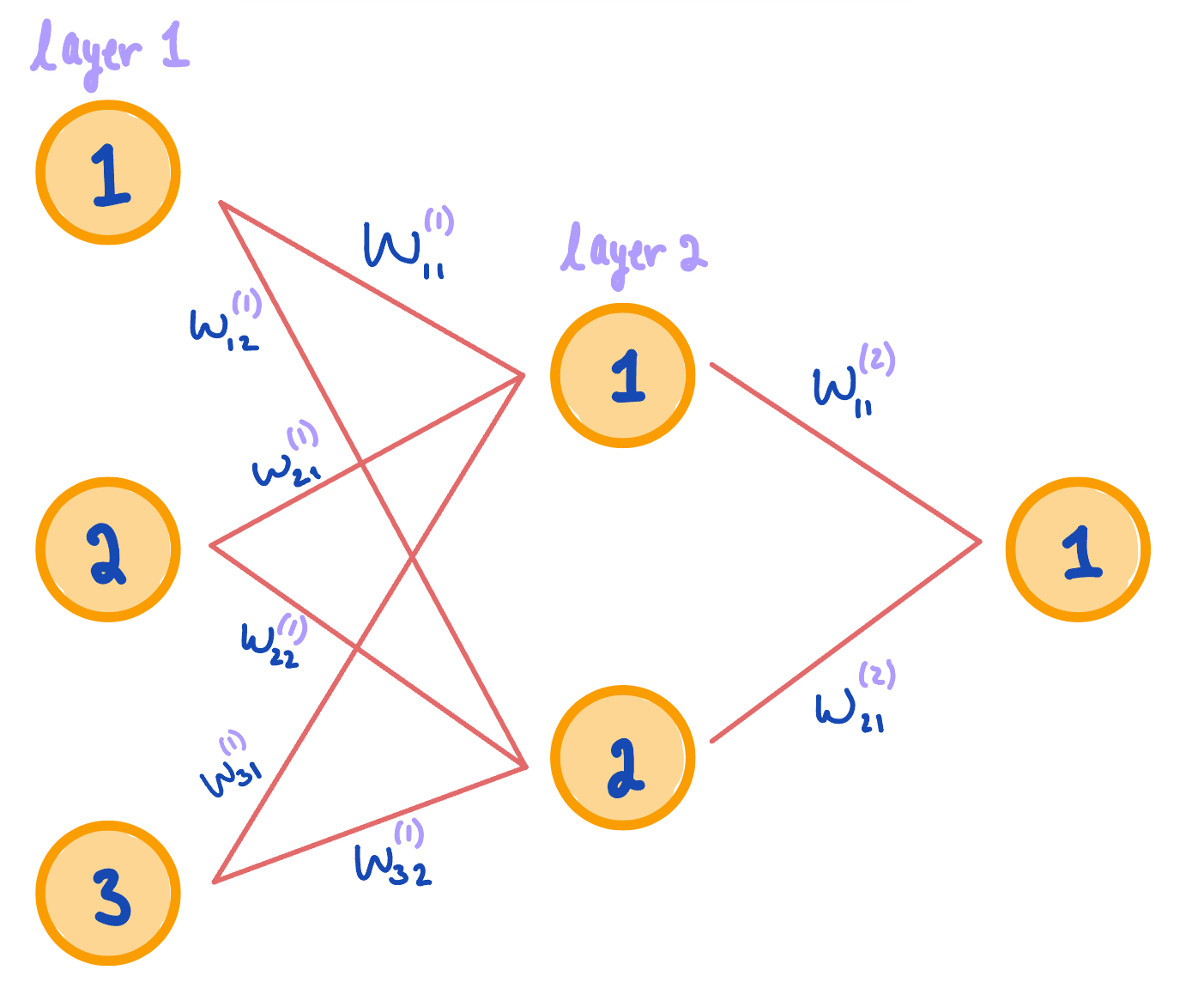
Figure 3. A diagram portraying the concepts of weight values used in neural networks. Subscripts specify node numbers. Superscripts specify layer numbers.

The first thing to understand is that each node communicates information via 'pathways' using weight values, \(W^{(i)}\), where \(i\) represents the layer. These weights range from (0, 1), exclusive. The greater the weight, the more important/relevant the pathway. Each pathway is expressed as a vector of weights. The length of these weight vectors depend on the number of nodes from one layer to the next. Consider the diagram above. Notice layer 1 has three nodes and layer 2 has two nodes. This means that there are 6 unique weight vectors containing 'information' in the form of real-numbered values ranging from (0, 1). The key is to optimize these values. In optimizing weight values, we optimize the transfer of information. We'll use partial derivatives to help us accomplish this in an algorithm called gradient descent, but more on that later. Since weights transfer information through the network, it makes sense the first weight matrix \(W^{(1)}\) directly involves the data we input \(X\). Thus, the output of our model \(z^{(i)}\) after transferring information from layer 1 to layer 2 is expressed as follows: $$z^{(2)} = XW^{(1)}$$ The next thing to understand is that each node has an activation function \(f(x)\). This function controls each node's magnitude of importance (i.e. weights). There are a few different activation functions that are used in neural networks, the two most common are the Sigmoid function and the ReLu function. Today, we will use the Sigmoid function because it is taught in a typical algebra course and thus more well known. Recall the Sigmoid function is an s-shaped curve that squishes real-numbered outputs such that the range is (0, 1), exclusive. This helps standardize the weight values. Each output matrix \(z^{(i)}\) is inputted into this activation function to recalculate and readjust weights at each layer of the network. We name this new output \(a^{(i)}\) to specify that it is the newly activated weights. Here it is mathematically: $$f(x) = \frac{1}{1 + e^{-x}}$$ $$a^{(2)} = f(z^{(2)})$$ Now that we understand the idea of weights, and how an activation function controls weights, we'll talk about bias terms, \(B^{(i)}\). Each and every node, except in the input layer, has a bias term. You can also think about it as each node that receives information has a bias term. These terms, similar to weights, are real-numbered values ranging (0, 1), exclusive. The difference being, instead of transferring information via pathways, bias terms transfer misinformation, or error. Including an error term as a part of every 'message' from one node to the next is our way to acknowledge the unavoidable uncertainty in the information propagated through our network. In essence, we are teaching the model humility. Mathematically, to include bias in our model, we simply add this bias matrix to the output matrix \(z^{(i)}\), as follows: $$z^{(2)} = XW^{(1)}+JB^{(1)^{T}}$$

There's some linear algebraic manipulation to make matrix dimensions compatible. Specifically, we take the dot product of the transpose of the bias matrix \(B^{(i)^{T}}\) with matrix of ones \(J=[1, 1,..., 1]\).

We continue this process until we reach the output layer. Once we reach the final output layer, the activation matrix is called the predicted output \(\hat{y}\). If we have only one hidden layer, then the entire forward propagation is expressed mathematically as follows: $$z^{(2)} = XW^{(1)}$$ $$a^{(2)} = f(z^{(2)})$$ $$z^{(3)} = a^{(2)}W^{(2)}+JB^{(2)^{T}}$$ $$a^{(3)} = f(z^{(3)})$$ $$\hat{y} = a^{(3)}$$ Okay, now it's time to focus on backward propagation - the process of feeding information backwards through our model. This is where the gradient descent algorithm comes into play. First let's talk about the loss function \(L\): $$(1)\;\;\; L = \sum (y - \hat{y})^2$$ $$(2)\;\;\; L = (y - \hat{y})(y - \hat{y})^{T} $$ \((3)\;\;\; L = (y - Xw)(y - Xw)^{T} \) , where \(w = [W^{(1)}, W^{(2)},...,W^{(i)}] \)

(1), (2), and (3) are mathematically equivalent. (1) uses sigma notation whereas (2) and (3) use matrix notation. (3) substitutes \(\hat{y}\) for \(Xw\). Since data frames are inherently matrices, we will use (3) in our coding algorithm.

This function will look familiar if you've taken an introductory statistics course. It is simply the sum of squared error between the actual output \(y\) and the predicted output \(\hat{y}\). We will implement this loss function to calculate the model's accuracy after forward propagation and before backward propagation. When the loss function is minimized, the propagation process stops and the model is optimized. The way we minimize the loss function is by implementing the gradient descent algorithm:

Gradient Descent Algorithm Methaphor. Imagine you are standing atop a mountain peak and wish to descend. You are blind so you cannot see the best way down and instead have to feel around you to determine which way descends the fastest, (in other words, which direction has the steepest slope). Once you identify the direction of steepest descent, you take one step in that direction. You repeat this process of feeling around, identifying the correct direction to move in, and taking a step in that direction. You repeat this process until you reach a point at which you can no longer identify a descending slope, signifying you are at the lowest point and have successfully descended.

Mathematically, to find the direction of steepest descent, we take the partial derrivative of the loss function \(L\) with respect to weights \(W^{(i)}\) and biases \(B^{(i)}\) as follows: $$(4)\;\;\;\; L = (y - Xw)(y - Xw)^{T} $$ $$(5)\;\;\;\; L = y^{T}y - 2w^{T}X^{T}y + w^{T}X^{T}Xw $$ $$(6)\;\;\;\; \frac{\partial L}{\partial w} = -2X^{T}y + 2X^{T}Xw $$

(4) is rewritten for convenience. (5) is the result of binomial expansion with matrix notation. (6) is the result of taking the partial derivative of (5).

Equation (6) calculates the direction of steepest descent. So now we need to 'take a step' in that direction. We use the learning rate \(\lambda\) to accomplish this. Recall that weights represent information, so in specifying a learning rate we specify how 'big of a step' we take in the direction of \(\frac{\partial L}{\partial w}\). Here's the math: $$ \Delta{F}(w) = \frac{\partial L}{\partial w} = [\frac{\partial L }{\partial W^{(1)}}, \frac{\partial L }{\partial W^{(2)}}, ..., \frac{\partial L }{\partial W^{(i)}}] $$ $$ w_{(i+1)} = w_i - \lambda\Delta{F}(w_i) $$ Where \(\Delta{F}(w_i)\) symbolizes the direction of steepest descent for step \(i\), and \(w_{(i+1)}\) symbolizes the upcoming step, where we take the current location \(w_i\) and descend toward \(\Delta{F}(w_i)\) at a rate of \(\lambda\). Note, for further detail, the partial derrivatives for each weight matrix is expressed as follows: $$\frac{\partial L }{\partial W^{(i)}} = a^{(i)^T}(-(y-\hat{y}) \odot f'(z^{(i+1)}) = a^{(i)^T} \delta_{i+1}$$ Okay, that's the end of backward propagation! To summarize, we start with the loss function calculated at the very end of forward propagation, then work backwards \(W^{(i)}, W^{(i-1)},W^{(i-2)},...,W^{(1)}\) finding the partial derivatives to optimize each layer's weights. The process of forward and backward propagation repeats until the weights and biases are optimized, resulting in the loss function being minimized, to finally halt the algorithm. Finally, once we have our optimal weights \(w = [W^{(1)}, W^{(2)},...,W^{(i)}] \) we push the data through our network one last time to predict the output \(\hat{y}\): $$ z^{(2)} = XW^{(2)} $$ $$ a^{(2)} = f(z^{(2)}) $$ $$ z^{(3)} = a^{(2)}W^{(3)} $$ $$ a^{(3)} = f(z^{(3)}) $$ $$ z^{(4)} = a^{(3)}W^{(4)} $$ $$ a^{(4)} = f(z^{(4)}) $$ $$...$$ $$ z^{(i)} = a^{(i-1)}W^{(i)} $$ $$ \hat{y} = f(z^{(i)}) $$

---

The Code

---

Forward Propagation

Recall, forward propagation is the process of information moving from the input layer to the output layer of an artificial neural network. We set up this process by initializing weights \(W^{(i)}\) with randomly generated values. This enables us to further initialize the output matrix \(z^{(i)}\) and activated values \(a^{(i)}\). It is okay to initialize with random guesses because through repeated forward and backward propagation, these values will be adjusted and optimized as the loss function is minimized.

									
######### Activation Function ######### 
sigmoid <- function(Z){
	1/(1 + exp(-Z))
}
										
######### Forward Feed - Initializing #########
W_1 <- matrix(runif(63), nrow = 21, ncol = 3)
Z_2 <- X %*% W_1
A_2 <- sigmoid(Z_2)
										
W_2 <- matrix(runif(9), nrow = 3, ncol = 3)
Z_3 <- A_2 %*% W_2
Y_hat <- sigmoid(Z_3)
									
								

Backward Propagation

Now that we have our matrices initialized, we can begin propagating forward and backward through the network, taking a step in the direction of steepest descent each time. Recall, the learning rate controls how far we move in the direction of steepest descent, or how big our 'step' is. If we make the learning rate too big (like 0.9) then our model will likely trust the direction too much and 'overstep', leading the model off course; too small, and our model will require many propagation interations to be optimized, which would be computationally expensive. The convergence boolean controls the number of propagation iterrations our model executes. When weight values are optimized, the algorithm halts.

									
######### Partial Derrivative of Activation Function  ######### 
sigmoidprime <- function(z){
	exp(-z)/((1 + exp(-z))^2)
}
								
######### Gradient Descent ######### 
learning_rate <- 0.01
W_1_old <- matrix(rep(0, 42), nrow = 21, ncol = 2)
converge <- FALSE
while(!converge){
  ## initialize weights, runs it through activation function, calculate y_hat
  Z_2 <- X %*% W_1
  A_2 <- sigmoid(Z_2)
  Z_3 <- A_2 %*% W_2
  Y_hat <- sigmoid(Z_3)

  ## find gradient
  delta_3 <- (-(Y - Y_hat) * sigmoidprime(Z_3))
  djdw2 <- t(A_2) %*% delta_3
  delta_2 <- delta_3 %*% t(W_2) * sigmoidprime(Z_2)
  djdw1 <- t(X) %*% delta_2

  ## update weights
  W_1 <- W_1 - learning_rate * djdw1
  W_2 <- W_2 - learning_rate * djdw2

  ## determine convergence
  w1round <- sum(round(W_1, 4))
  w1round_old <- sum(round(W_1_old, 4))
  if(w1round != w1round_old){
    W_1_old = W_1
  }else{
    converge = TRUE
  }
}
								

That's it! Using the coded algorithm above, we found the optimal weights. Testing the accuracy of our predictions using cross-validation, this model is about 84% accurate overall in its predictions.

---

Diabetes Status Calculator

---

Below, I created a form for you to input data and run it through our algorithm to calculate diabetes risk. Play around with values to explore which variables have the highest inluence on type 2 diabetes development!

1. What is your sex?

Male Female

2. Do you have difficulty walking or climbing stairs?

Yes No

3. Do you have healthcare coverage, including health insurance, prepaid plans such as HMO, etc.?

Yes No

4. Is there a time in the past 12 months when you needed to see a doctor but could not because of cost?

Yes No

5. Do you have hypertension (high blood pressure)?

Yes No

6. Do you have high cholesterol?

Yes No

7. Have you had your cholesterol checked in the last 5 years?

Yes No

8. Have you smoked as least 100 cigarettes in your life? [Note: 5 packs = 100 cigarettes]

Yes No

9. Have you ever had a stroke?

Yes No

10. Have you had coronary heart disease (CHD) or myocardial infraction (MI)?

Yes No

11. Have you been physically active in the past 30 days?

Yes No

12. Do you consume at least 1 fruit a day?

Yes No

13. Do you consume at least 1 vegetable a day?

Yes No

14. Do you consume heavy amounts of alcohol? For men this means having more than 14 drinks per week. For women, this means having more than 7 drinks per week.

Yes No

15. What is your BMI?

Value:

16. What is your Income?

• 1 = less than $10,000
• 2 = between $10,000 and $15,000
• 3 = between $15,000 and $20,000
• 4 = between $20,000 and $25,000
• 5 = between $25,000 and $35,000
• 6 = between $35,000 and $50,000
• 7 = between $50,000 and $75,000
• 8 = more than $75,000

Value:

17. What is your highest level of Education?

• 1 = None
• 2 = Elementary
• 3 = Some High School
• 4 = High School Graduate
• 5 = Some College or Technical School
• 6 = College Graduate

Value:

18. How many days in the past month have you experienced physical illness and/or injury?

Value:

19. What is your personal ranking of your General Health?

• 1 = Excellent
• 2 = Very Good
• 3 = Good
• 4 = Fair
• 5 = Poor

Value:

20. How many days in the past month have you experienced feelings of stress, depression, and problems with emotions?

Value:

21. What is your age?

Value:

Submit

Disclaimer. This calculator should not be trusted blindly so please consult a medical professional for credible and trustworthy claims. Also, I will not collect, track, nor save any data entered in this form.

---

Abstract

---

[1] NIH Diabetes Facts and Statistics

[2] CDC Diabetes Information

[3] Neocortical neuron number in humans: effect of sex and age

[4] Prerequisite Mathematical Knowledge guide

1. Calculus - Partial Derivatives

2. Linear Algebra - Operations

[5] The values in the W_1 matrix. This cab be used to interpret magnitude of influence each predictor has on diabetes risk.