An Introduction to R
Jan 15, 2024
Lecture Outline
- RStudio IDE
- Arithmetic, Syntax, and Basics
- Class Types
- integer | numeric | logical | character | matrix | data frame
- Linear Algebra
- Functions
- Loops
- Simulating and Importing Data
- Visualizing Data
- scatterplot | histogram | boxplot | barplot | pie chart | line graph
- Modeling Data - Regression
- lm() | linear | quadratic | cubic | poly() | mean squared error (MSE)
- Modeling Data - Classification
- Final Exercises
- Appendix
RStudio
RStudio is an integrated development enviornment (IDE) for R. It is one of the most common R programming environments for data scientists. If you don't already have RStudio downloaded on your computer, please download the free desktop version here: RStudio download. We will be actively programming throughout the lesson.
[Command] + [enter] - Runs current line
[Command] + [s] - Saves file
[Command] + [l] - Clears console
Tools -> Global Options -> Appearance -> Editor Theme - To change the overall appearance
Arithmetic, Syntax, and Basics
Basic mathematical operations in R, including the assignment of variables, naming convenctions, and traditional syntax. Notable functions used in this section inlcude:
- sum( ) - sum function with a vector as the input
- mean( ) - mean/average function with a vector as the input
- log( ) - logarithmic function: \(\log_{10}(x)\)
- exp( ) - exponential function: \(e^{x}\)
- sqrt( ) - square root function \(\sqrt{x}\)
- round( ) - rounding function: \(round(a, b)\), where the real number \(a\) is rounded to \(b\) decimal places
######## Assigning Variables ########
x <- 2
x = 2     #Note "=" often works but "<-" is the convention for R
y <- 3
b <- 2
z <- 3.12345
s <- "Welcome!"

adding <- x + y
sum(x, y)
subtracting <- x - y
multiplying <- x * y
dividing <- x / y
exponents <- x^b
square_root <- sqrt(x)
logarithms <- log(x)
exponentials <- exp(x)
mean(c(x, y))

rounding <- round(z)
rounding1 <- round(z, 1)
rounding2 <- round(z, 2)

######## R Naming Convention: snake_case ########
variable_name <- 523
variable_name

pls.dont.use.dots.even.tho.it.works <- 3049
pls.dont.use.dots.even.tho.it.works
Class Types
We will specify 5 class types in this section: numeric, logical, character, matrix, data frame. Notable functions/operations used in this section inlcude:
- c( ) - combines elements into a single vector
- seq(from = a, to = b, by = c) - sequence function, where \(a, b,\) and \(c\) specify the beginning, end, and incriment, respectively
- a:b - creates a sequence from \(a\) to \(b\), incrimenting by 1
- seq_len(b) - creates a sequence from 1 to b, incrimenting by 1. More suitable for interative loops
- matrix(n, nrow = a, ncol = b) - creates a matrix, must specify elements \(n\), number of rows \(a\), number of columns \(b\)
- data.frame( ) - creates a data frame with a matrix or vectors as the input
- class( ) - returns the class type of the input
######## Numeric ########
a_numeric <- 456
another_numeric <- 12.367
yet_another_numeric <- pi

a_vector <- c(1, 2, 3, 4)
a_sequence <- seq(from = 10, to = 100, by = 10) 	# an ordered list of numbers
another_sequence <- 1:10 				# Integer
yet_another_sequence <- seq_len(10)		# A sequence suitable for loops

######## Logical ########
a_boolean <- 2 == 3
another_boolean <- 1 + 2 == 5 - 2
sum(a_boolean)
sum(another_boolean)

######## Characters ########
a_charater <- "Hello"
another_character <- 'Datafest!'

######## Matrix ########
a_matrix <- matrix(1, nrow = 2, ncol = 5) 		# a Matrix-Array
a_more_interesting_matrix <- matrix(a_sequence, nrow = 2, ncol = 5)

######## Data Frame ########
a_dataframe <- data.frame(a_matrix)

######## Testing Class Types with class() ########
class(a_numeric)
class(another_numeric)
class(yet_another_numeric)
class(a_vector)
class(a_sequence)
class(yet_another_sequence)
class(a_matrix)
class(a_boolean)
class(a_charater)
class(a_dataframe)
Linear Algebra
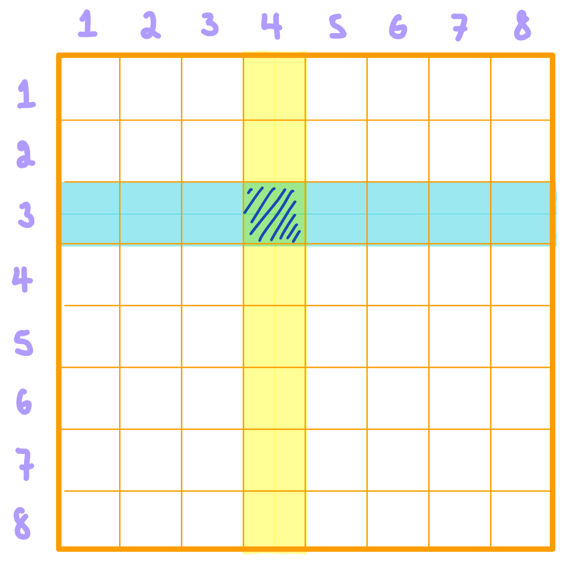
Matrices are described by two dimensions: row \((m)\) and column \((n)\). If a matrix has 2 rows and 3 columns, we say it is a "two by three matrix," denoted as \( m \times n\). We use capital letters to name matrices. If we name the above matrix, \(A\), we can say \(A\) is a \(8 \times 8\) matrix. Each individual cell within a matrix is called an element. Elements are referred to using their location within the matrix they belong to. Using matrix \(A\) as an example, the overlapped highlighted element is located at the row index = 3 and column index = 4, so this element is denoted as \(A[3, 4]\). If we wanted to refer to all the elements in column 4, we would denote this as \(A[\hspace{0.2cm}, 4]\), leaving a blank space in the row placeholder. Similarly, we would write \(A[3,\hspace{0.2cm}]\) to refer to all the elements in row 3 of matrix \(A\).
Vectors are one dimensional matrices - either the row dimension = 1 or the column dimension = 1.
Notable functions/operations used in this section inlcude:
- cat( ) - concatenate function
- t( ) - transpose function
- length( ) - returns the length of a vector
- dim( ) - returns the dimensions of a matrix or data frame
- head(a, b) - prints the first \(b\) rows of vector/matrix/data frame \(a\)
- View( ) - shows a matrix/data frame in an asthetic viewer display
######## Vectors ########
num_vector <- c(1, 2, 3, 4, 5, 6, 7)
char_vector <- c("D", "a", "t", "a", "f", "e", "s", "t", "!")
x <- num_vector[1]
y <- char_vector[4]
sum(x, y)
char_vector
cat(char_vector)
length(char_vector)

######## Matrices ########
a_matrix <- matrix(data = seq(from = 1, to = 20, by = 1),	#note, we are using "=" here
                   nrow = 10,
                   ncol = 2)
a_matrix
row <- 5
col <- 2
a_matrix[row, col]
a_matrix[1, ]              #1st row, all columns
a_matrix[, 1]              #All rows, 1st column
a_matrix[1, 1] <- 75       #rewrite the 1st row 1st column element to = 75

mean(a_matrix) 		   #average
t(a_matrix)    		   #transpose
dim(a_matrix)  		   #dimensions

number_of_rows_displayed <- 3
head(a_matrix, number_of_rows_displayed)  #displays top rows

View(a_matrix)    #displays matrix in spreadsheet format
Functions
Functions accept an input, perform specified tasks and/or return an output as a response dependent on the input value(s). Notable functions/operations used in this section include:
- if( ) - conditional function
- else if ( ) - conditional (local) contingency function
- else( ) - conditional (absolute) contingency function
- print( ) - prints input to the console
- return( ) - return function
- install.packages( ) - installs packages not yet downloaded to your PC
- library( ) - calls packages already downloaded to your PC
- |> - a pipeline operator that chains a sequence of calculations/tasks
- %>% - alternative notation for pipeline operation using the dplyr library
- mutate( ) - adds new variable or rewrites an old variable, within a data frame
- summarise( ) - aggregates variables using summary statistics (i.e mean, median)
- group_by( ) - groups a data frame by the levels of a specified variable
######## IF/ELSE Conditional Function ########
if(1 > 10){
  print("If 1 > 10 is TRUE, then this will print!")
} else if(80 == 40 * 2) {
  print("Cool, 80 is equal to twice of 40!")
} else{
  print("Darn, they were all false so now you have me!")
}


######## Functions ########
a_summation_function <- function(a, b){
  return(a + b)
}
a_summation_function(5, 11)


######## Pipelines ########
install.packages("dplyr")
library(dplyr)

pipe_ex <- 1:10
pipe_ex |> sum()
pipe_ex %>% mean()
pipe_ex |> order(decreasing = TRUE)

pipe_ex2 <- data.frame(numbers = sample(1:100, 8),
                       letters = c("A", "B", "B", "A", "C", "A", "B", "A") )

pipe_ex2 |>
  group_by(letters) |>
  summarise(sum = sum(numbers))

pipe_ex2 |>
  mutate(new_var = numbers * 10)
Checkpoint 1: Write a function that computes the nth power of base b
Challenge: Write a function that computes the euclidean distance between two points (x1, y1) and (x2, y2)
Loops
Loops describe iterative and/or repetitive functions. Notable functions and operations used in this section include:
- for(i in a:b ) - for loop, must specify iterative index variable \(i\), and the sequence to loop through \(a:b\)
- while(condition) - while loop, input is a boolean
- paste0( ) - concatenates vectors into a string
######## For Loops ########
for(i in seq_len(10)){
  print(2 * i)
}

datafest <- c()
for(i in 1:20){
	datafest[i] <- "datafest"
}
datafest

######## While Loops ########
count <- 1
while(count <= 5){
  print(paste0("This repeats until count equals 6. We're currently on iteration ", count, "."))
  count <- count + 1
}
Checkpoint 2: Write a loop that outputs the first 50 terms of the Fibonacci Sequence
Challenge: Write a loop that outputs the first 100 terms of the following sequence: 4, 9, 16, 25, 36, ...
Simulating and Importing Data
We will begin to work with data in this section, focusing on creating and importing data. We will be importing the following csv file: music.csv 1. Notable functions/operations used in this section include:
- set.seed(a) - function to allow for reproducibile random generator values, inputs an integer \(a\)
- runif(n, min = , max = ) - random number generator following a uniform distribution
- rnrom(n, mean = , sd = ) - random number generator following a normal distribution
- read.csv("path") - imports .csv file, input is the file path
- dataframe$x - calls the column name \(x\) of a dataframe
######## Simulating Non-Random Data ########
seq(from = 1, to = 10, by = .5)
1:10
######## Simulating Random Data ########
set.seed(1) #for reproducibility when using a random generator
runif(n = 10, min = 0, max = 100) #random uniform #'s
rnorm(n = 10, mean = 0, sd = 1) #random normal #'s
runif(10, 0, 100) #you don't always have to specify the function - check defaults
######## Importing Data ########
install.packages("dplyr")
imported_data <- read.csv("~/Desktop/music.csv")
View(imported_data)
######## Data Frames ########
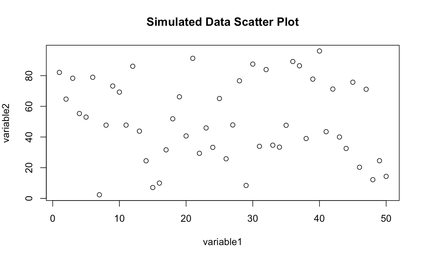
a_dataframe <- data.frame(x1 = 1:50,
x2 = runif(50, 0, 100))
a_dataframe
View(a_dataframe)
a_dataframe$x1 #calls the vector named x1 from a_dataframe
Visualizing Data
We will produce many different types of plots and graphs in this section, including: scatter plot, line graph, histogram, bar plot, box plot, pie chart.
Scatter Plots and Line Graphs
-
plot( ) - generic plot function to display coordinate grid plot
- x - x coordinates
- y - y coordinates
- type = "" - specifies graph type: "p" - point, "l" - line, "b" - both
- main = "" - main title
- xlab = "" - x axis label
- ylab = "" - y axis label
- xlim = c(a, b) - x axis scale ranging from a to b
- ylim = c(a, b) - y axis scale ranging from a to b
- col = - specifies color
- lwd = a - specifies line width with real number a
- cex = a - specifies point size with real number a
- pch = a - specifies point type with whole number a
- lines( ) - displays a line segment given (x, y) coordinates. Similar parameter options as plot( )
- legend( ) - manually produces a legend on your plot
- locator - location of legend, can specify (x, y) coordinate or verbal location like "topleft
- legend - specifies label names
- fill - specifies color asthetics
plot(x = 1:10, y = 1:10, main = "Scatter Plot")
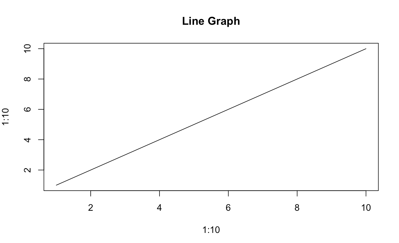
plot(x = 1:10, y = 1:10, type = "l", main = "Line Graph")
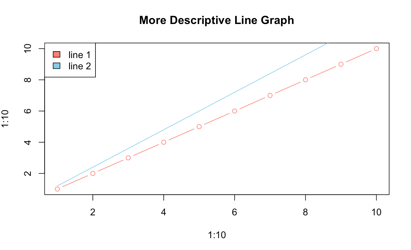
plot(x = 1:10, y = 1:10, type = "b", col = "salmon", main = "More Descriptive Line Graph")
lines(x = 1:10, y = 1.2*(1:10), col = "skyblue")
legend("topleft",
legend = c("line 1", "line 2"),
fill = c("salmon","skyblue"))
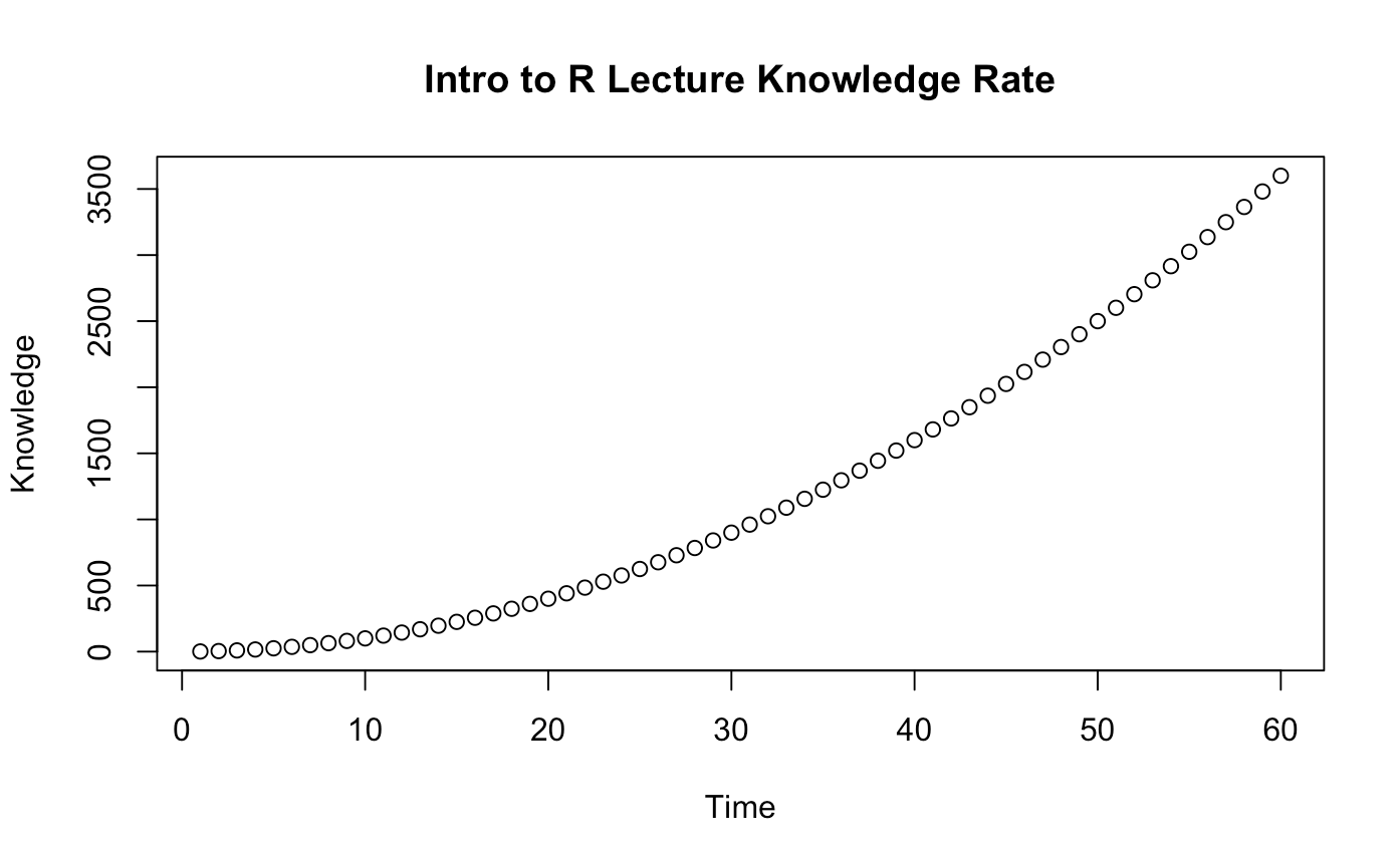
plot(x = 1:60, y = (1:60)^2,
type = "b",
main = "Intro to R Lecture Knowledge Rate",
xlab = "Time", ylab = "Knowledge")
plot(a_dataframe, main = "Simulated Data Scatter Plot")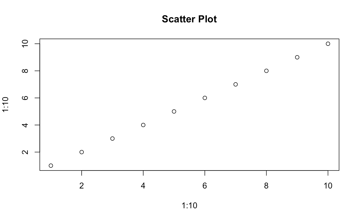
Histograms
- hist( ) - creates a histogram given a vector. Similar parameters as plot( ) except you only specify \(x\)
hist(x = rnorm(10, mean = 0, sd = 1)) #Note: default is mean = 0, sd = 1
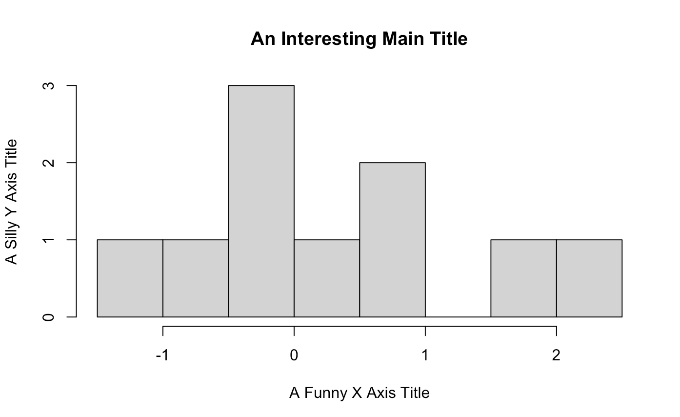
hist(x = rnorm(10),
main = "An Interesting Main Title",
xlab = "A Funny X Axis Title",
ylab = "A Silly Y Axis Title")
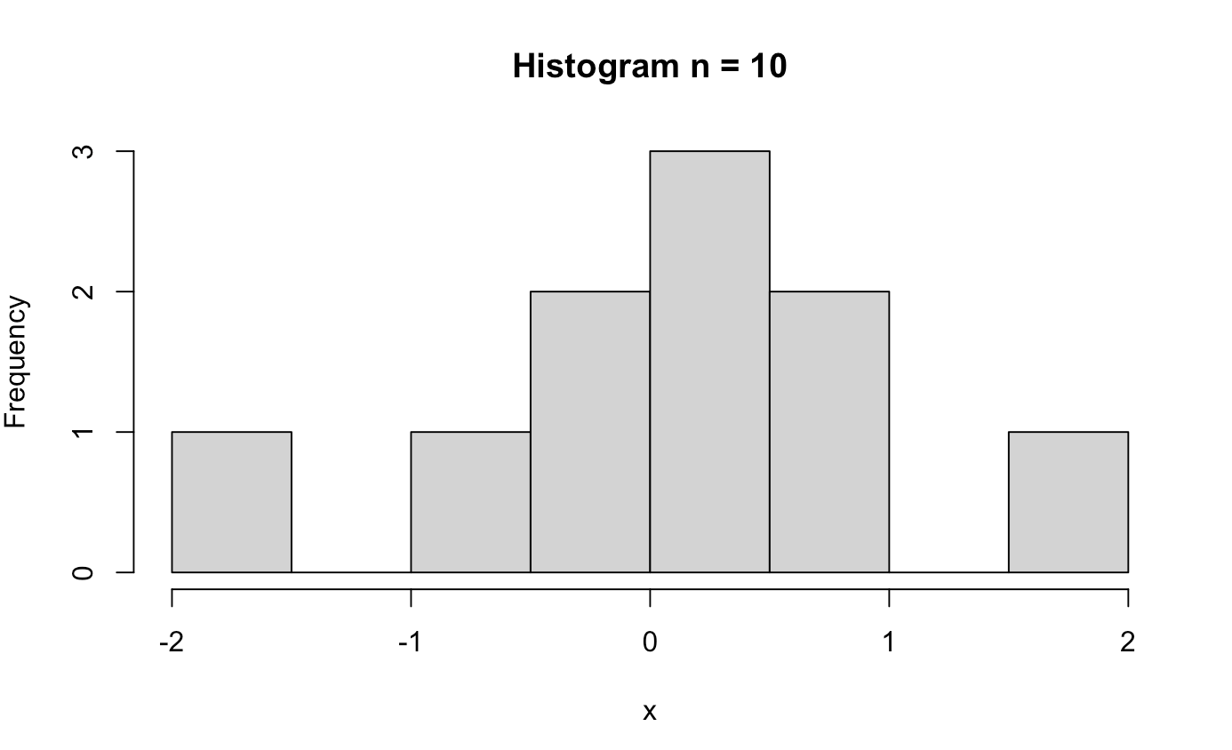
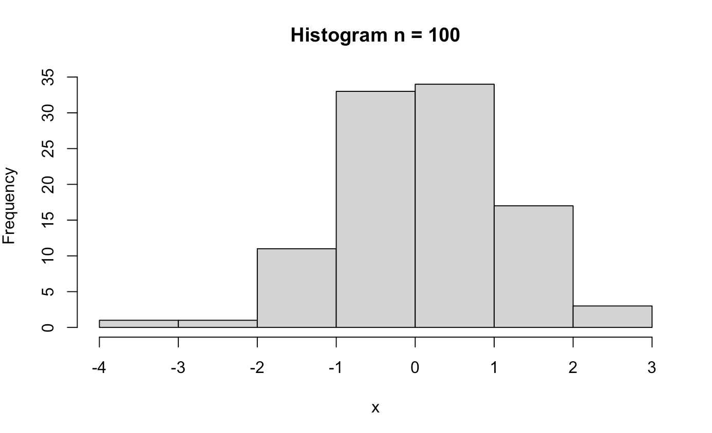
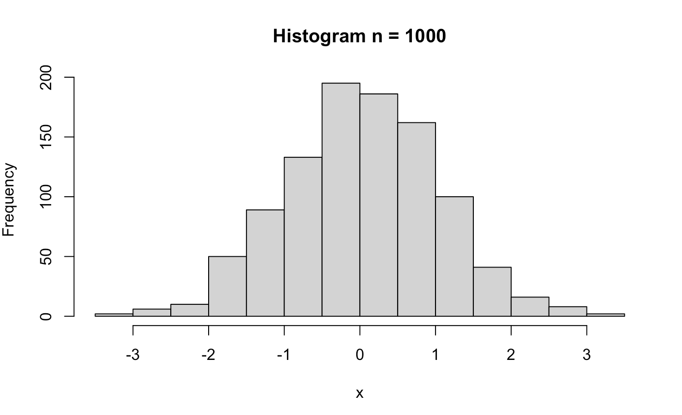
######## Central Limit Theorem ########
clt_test <- function(n){
x <- rnorm(n)
hist(x, main = paste0("Histogram n = ", n))
}
clt_test(10)
clt_test(100)
clt_test(1000)
clt_test(10000)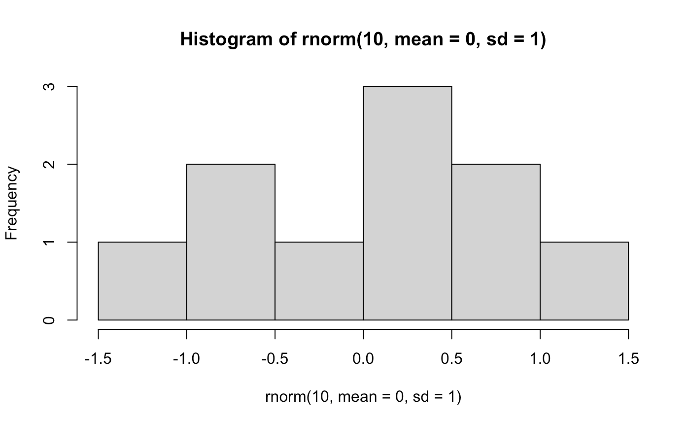

Bar Plot
- barplot( ) - creates a barplot given height values
- height - specifies height values for each bar
- names - specifies label names for each bar
- horiz - boolean to control layout: "TRUE" - horizontal layout, "FASLE" - vertical layout
- las = a - orients axis labels with whole number \(a\) raging [0-3]
- cex.names = a - x axis label with real number \(a\)
barplot(height = 1:10)
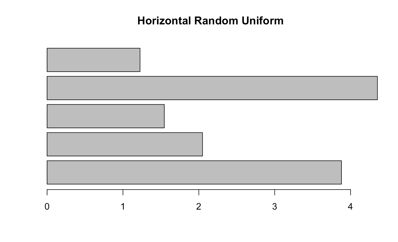
barplot(height = runif(5, 0, 10),
horiz = TRUE)
barplot(height = c(52, 45, 67, 36, 46),
names = c("Watermelon Sugar", "Adore You", "Golden", "She", "As It Was"),
horiz = TRUE,
las = 1,
cex.names = 0.5,
col = c(1, 2, 3, 4, 5),
main = "What Would You Name The Main Title?")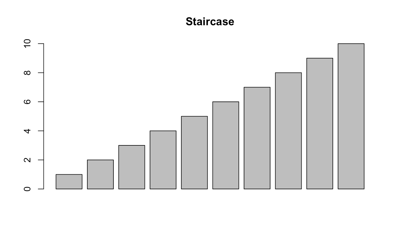
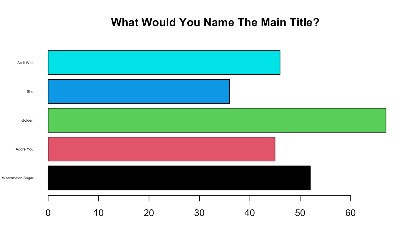
Checkpoint 2: Come up with a descriptive title for the bar graph above.
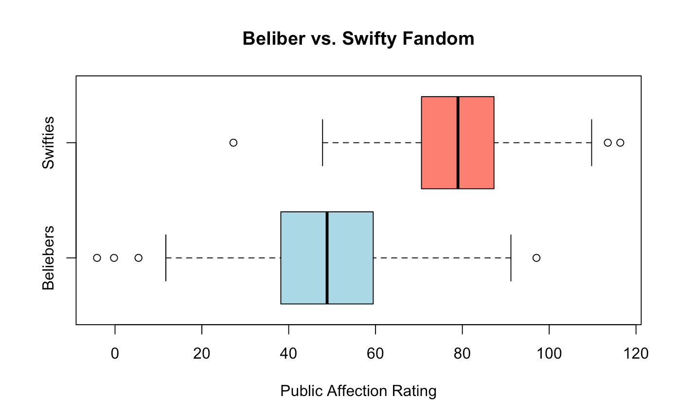
Box Plot
- boxplot(v1, v1, ..., v3) - creates a boxplot for each vector inputted
bieber_fandom <- rnorm(100, mean = 50, sd = 20)
swift_fandom <- rnorm(100, mean = 80, sd = 15)

boxplot(bieber_fandom, swift_fandom)

boxplot(bieber_fandom, swift_fandom,
        names = c("Beliebers", "Swifties"),
        main = "Beliber vs. Swifty Fandom",
        xlab = "Public Affection Rating",
        horizontal = TRUE,
        col = c("lightblue", "salmon"))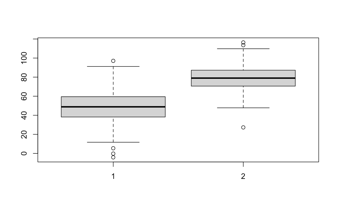
Real Data
- table( ) - creates a table of count values, given a vector
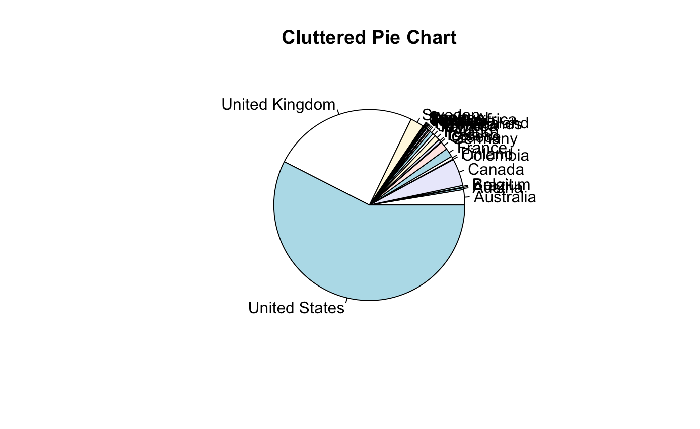
- pie( ) - creates a pie chart given a vector of count values
- order( ) - sorts values in ascending/descending order, given a vector
######## Music Data ########
music <- imported_data
dim(music)
View(music)
table(music$country)
barplot(height = table(music$country), main = "Artist Count by Country")
pie(table(music$country), main = "Cluttered Pie Chart")
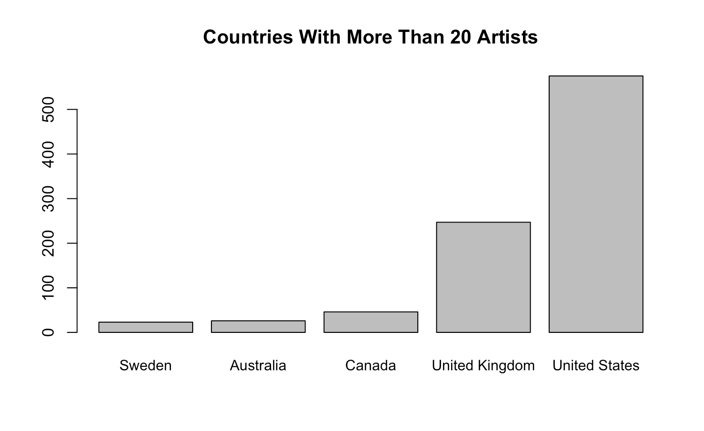
## So many countries! Let's remove the smaller ones
country_table <- table(music$country)
View(country_table)
country_table <- country_table[country_table >= 20]
country_table <- country_table[order(country_table)]
barplot(country_table, main = "Countries With More Than 20 Artists")
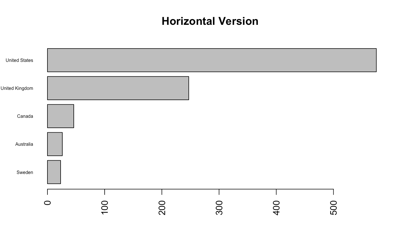
barplot(country_table, horiz = TRUE, las = 2, cex.names = 0.5,
main = "Horizontal Version")
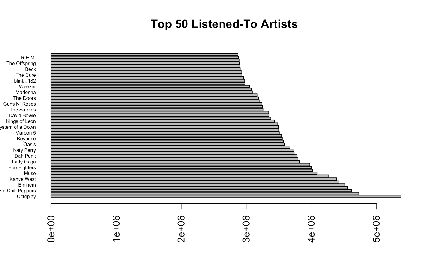
## Lets compare the top 50 artists
barplot(height = music$listeners[1:50],
names = music$artist[1:50],
horiz = TRUE,
las = 2,
cex.names = 0.5,
main = "Top 50 Listened-To Artists")
## Searching for specific artists
which(music$artist == "Taylor Swift")
which(music$artist == "Justin Bieber")
music[138, ]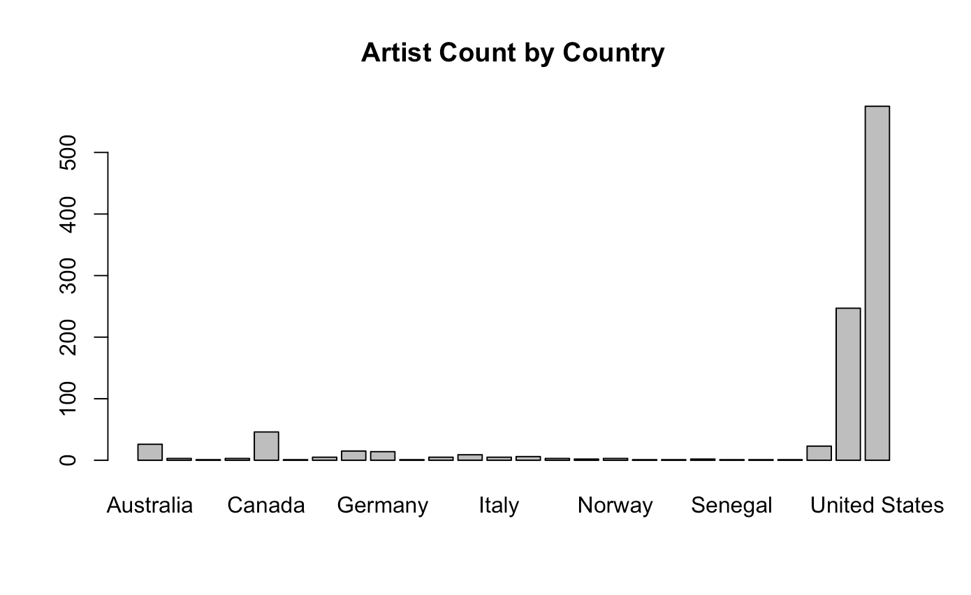
Modeling Data - Regression
We will fit a few different functions to model data for regression, inlcuding: linear, quadratic, and cubic. We will be importing the following csv file: cookies.csv. Notable functions/operations used in this section include:
- lm(y ~ x, data) - linear model fitting function, must specify independent variable(s) \( x_1, x_2, ..., x_n\), response variable \(y\), and data frame
- predict(model, newdata) - creates numerical predictions for new independent variables in newdata, given a model
- summary(model) - prints attributes of a fitted model, including coefficients and accuracy metrics
- I( ) - specifies to R that a predictor should be used 'as-is' and as expected
- which(condition) - finds indices for which a logical condition is true
######## Create Data ########
data <- data.frame(x = 1:10, y = (1:10)^2) # y = x^2 for 1 < x < 10
plot(data)
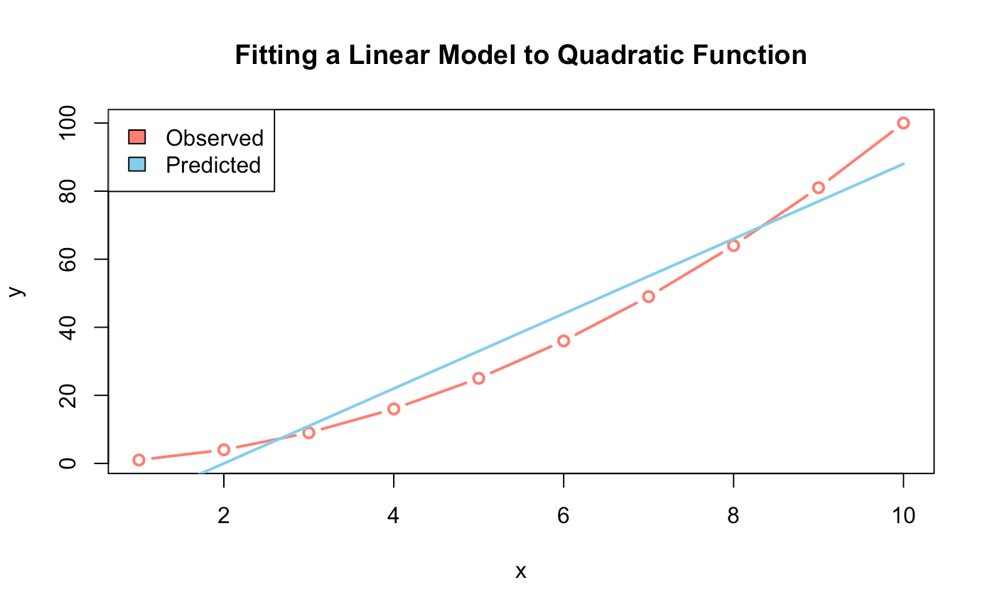
######## Linear Regression Model lm() ########
lin_model <- lm(y ~ x, data = data)
predict_lin_model <- predict(lin_model)
summary(lin_model)
## Plotting ##
plot(data,
type = "b",
col = "salmon",
lwd = 2,
main = "Fitting a Linear Model to Quadratic Function")
lines(predict_lin_model, col = "skyblue", lwd = 2)
legend("topleft",
legend = c("Observed", "Predicted"),
fill = c("salmon","skyblue"))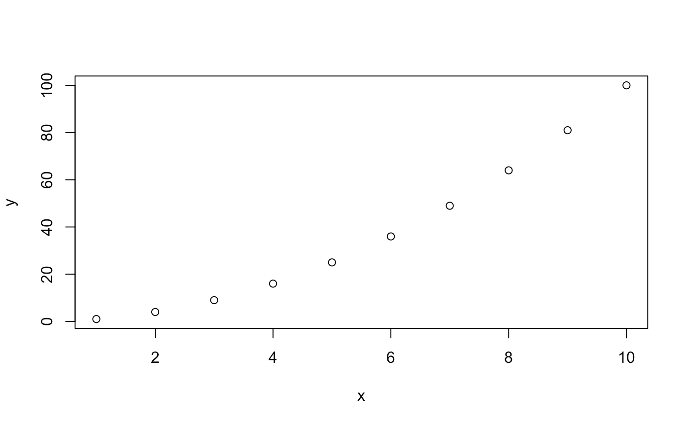
######## Quadratic Model ########
quad_model <- lm(y ~ I(x^2), data = data)
predict_quad_model <- predict(quad_model)

plot(data,
     type = "b",
     col = "salmon",
     lwd = 2,
     main = "Fitting a Quadratic Model to Quadratic Function")
  lines(predict_quad_model, col = "skyblue", lwd = 2)
  legend(x = 2, y = 90,
         legend = c("Observed", "Predicted"),
         fill = c("salmon","skyblue"))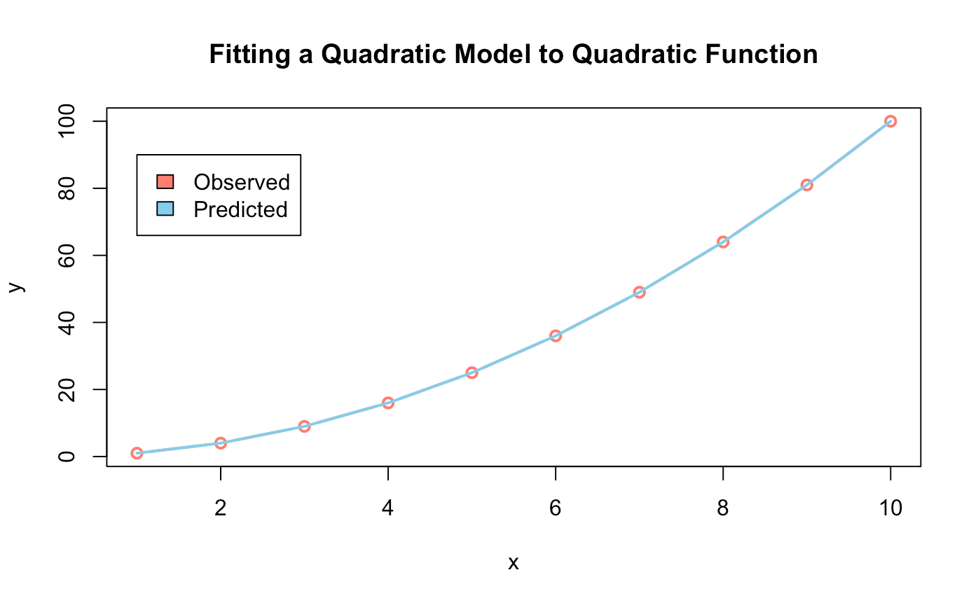
######## Cubic Model ########
cubic_model <- lm(y ~ I(x^3), data = data)
predict_cubic_model <- predict(cubic_model)

plot(data,
     type = "b",
     col = "salmon",
     lwd = 2,
     main = "Fitting a Cubic Model to Quadratic Function")
  lines(predict_cubic_model, col = "skyblue", lwd = 2)
  legend(x = 2, y = 90,
         legend = c("Observed", "Predicted"),
         fill = c("salmon","skyblue"))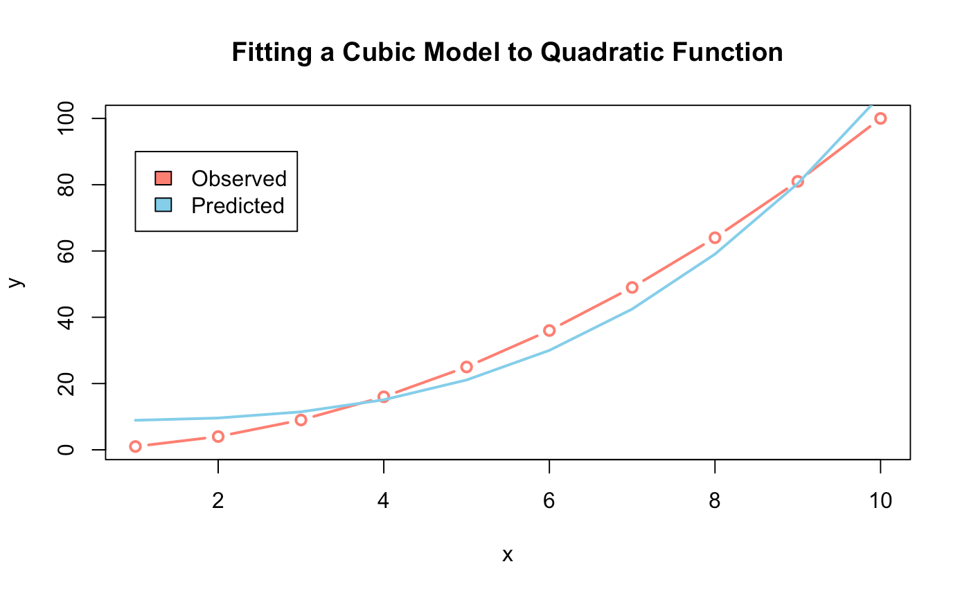
Checkpoint 3:Challenge: Write a function to compute the MSE
- Read in the cookies.csv file
- Fit a linear model to the data
- Predict the number of cookies I will eat on the 7th day
- Plot the actual data and fitted model on the same graph, make it asthetically descriptive
Modeling Data - Classification
We won't cover classification methods here, but check out my article on Breast Cancer Detection for an instructive walkthough. In this article, I use logistic regression to classify breast cancer tumors as malignant or benign.
Final Exercise
- Choose one of the following data sets*:
- Explore the data set: plot(), summary(), dim(), View()
- Fit a model to the data: lm()
- Calculate predictions: predict()
- Create a visual of the observed data and fitted model: plot()
- Calculate accuracy of your model using MSE
*You're welcome to look for other data sets on kaggle, data.gov, etc.
Appendix
Here you can find answers to the checkpoint exercises.
- Power Function
- Euclidean Distance Function
- Write a loop that stores the first 100 terms of the following sequence: 4, 9, 16, 25, 36, ...
- Write a loop that outputs the first 50 terms of the Fibonacci Sequence
- Cookies Regression Analysis
- MSE Function
power <- function(b, n){     # b^n
  print(b^n)
}
power(5, 2)euclidean_distance <- function(point1, point2){ # a^2 + b^2 = c^2
horiz_vert_dist <- (point1 - point2)^2
add_them_up <- sum(horiz_vert_dist)
return(sqrt(add_them_up))
}
xy1 <- c(0, 0)
xy2 <- c(1, 1)
euclidean_distance(xy1, xy2)terms <- c()
terms[1] <- 4
for(i in 1:100){
terms[i + 1] <- terms[i] + 2*i + 3
}
termsfib <- c()
fib[1] <- 0
fib[2] <- 1
for(i in 3:50){
fib[i] <- fib[i - 1] + fib[i - 2]
}
fib# Step 1: read in data
cookies_df <- read.csv("~/Desktop/cookies.csv")
# Step 2: plot raw data to observe the shape
plot(cookies_df)
# Step 3: fit linear model
cookies_model <- lm(Cookies ~ Day, data = cookies_df)
# Step 4: predict day 7 using cookies model
predict_cookies <- predict(cookies_model, newdata = data.frame(Day = 1:7))
predict_cookies[7]
# Step 5: Plot
plot(cookies_df,
type = "b",
col = "salmon",
lwd = 2,
main = "Cookies Linear Regression Model Actual vs Fitted")
lines(predict_cookies, col = "skyblue", lwd = 2)
legend("topleft",
legend = c("Observed", "Predicted"),
fill = c("salmon","skyblue"))
points(x = 7, y = predict_cookies[7], col = "red", pch = 16)
text(x = 7, y = predict_cookies[7]+0.3, paste0(predict_cookies[7]))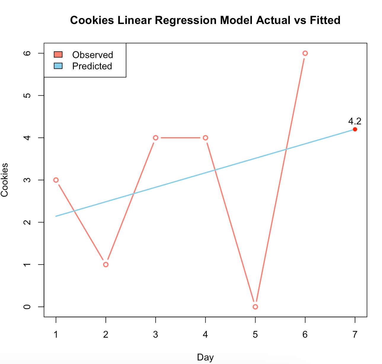
mse <- function(y, yhat){
  error <- mean( (y - yhat)^2 )
  return(error)
}

mse(data$y, predict_lin_model)
mse(data$y, predict_quad_model)
mse(data$y, predict_cubic_model)